Welcome to my website! I am a researcher originally from San Diego with interests in latent world models, self-supervised learning, and physics. Currently, I'm working on identifying failure cases of frontier models and building evaluations for them.
I hold an Sc.B. in Biophysics and an Sc.B. in Applied Math-Computer Science from Brown University. During this time, I did world model research with Randall Balestriero as part of the GalilAI lab, and I did machine learning research at CERN as part of the CMS project with Loukas Gouskos.
I'm into music, fantasy books, and video games. My favorite band is The Red Hot Chili Peppers and I'm deep into Brandon Sanderson's Cosmere universe. Some of my favorite games include Hollow Knight, Outer Wilds, and The Stanley Parable. I also play ice hockey (there are ice rinks in San Diego, believe it or not), and I love to ski and wakesurf!
2022–26sc.b. biophysics — brown university2022–26sc.b. applied mathematics–computer science — brown university2018–22francis parker school — san diego
honors theses
2026continual learning with latent world modelsadvised by randall balestriero — galilai lab2026jet flavour tagging with archived aleph dataadvised by loukas gouskos — cms @ cern
distinctions
2026honors in physics2026honors in applied math–computer science2026magna cum laude2026mildred widgoff prize for excellence in thesis preparation (physics)
Mechanistic interpretability on a chess transformer model
[1] overview
When I started this project, I set the goal is to build a gpt type model that plays chess, then do interpretability on this to demonstrate various mechanistic interpretability concepts.
I have three phases for this project. At the time of writing this, two of them are completed.
Pretraining: build and train the model
Probing: take the pretrained model and learn a linear probe of various points in the residual stream for things like board position, existence of tactics, and more
Intervention: using the probes, intervene in certain states to adjust the models board state, tendency to predict and act on tactics, and maybe more. It would be great if I could create an interactive model here where I could intervene on the fly and see the effect.
[2] pretraining
data — source
For pretraining and some probing, I am using chess games pulled from the Lichess hugging face dataset. I filter for games in which there are at least 15 moves and both players have an elo of at least 1800. In total, I pull around 40,000 games.
data — format
Ad described below, I structure our model to take in the series of moves up to the current state instead of the current board state. On most chess websites, books, and tournaments you will see moves written in Standard Algebraic Notation (SAN). However, most computational chess models use a different format that is part of the Universal Chess Interface (UCI). While the Lichess database is in SAN, we translate this is UCI and use this as input to our model.
data — tokenization
UCI moves are structured as [square the piece is moving from][square the piece is moving to]<promotion>. Castles can be represented in this format as moving the king to the location after castle.
task
Chess is, aside from modeling player behavior, Markovian. When deciding on a move, what matters is the current position not the sequence of moves that led there. This means the strongest formulation of a chess prediction task would take the current board state as input and predict the best move, essentially learning a value function over positions.
But that's not the formulation I chose. My goal is to learn about mechanistic interpretability through models that resemble large language models. To mimic the self-supervised next-token prediction paradigm of LLMs, I instead frame the task as sequence prediction: given the moves played so far, predict the next move.
Formally, given a sequence of moves {m₁, m₂, …, mₙ}, the model learns a function f that takes {m₁, m₂, …, mₖ} and predicts mₖ₊₁. Just as language models can extract n−1 training examples from a single sentence of length n (by masking increasingly longer prefixes), I extract n−1 training examples from each chess game.
This formulation has an interesting implication: the model must implicitly reconstruct the board state from the move sequence. It cannot simply "look" at the current position. Instead, it must track how each move transforms the board. This makes the internal representations potentially richer and more interpretable.
model
The architecture is a GPT-style transformer based on NanoGPT. The pipeline consists of:
Embedding layer: Maps tokens to dense vectors and adds positional encodings
Transformer blocks: 12 layers, each containing:
Multi-head self-attention
Feed-forward MLP
Layer normalization and residual connections
Output head: Projects the final hidden state to a probability distribution over all possible tokens
In total, it is only 88.M parameters. The model outputs a probability distribution across all moves in the vocabulary. During inference, the predicted move is simply the one with the highest probability.
The model was trained using cross-entropy loss, comparing the predicted probability distribution against the actual next move played in each game.
evaluation
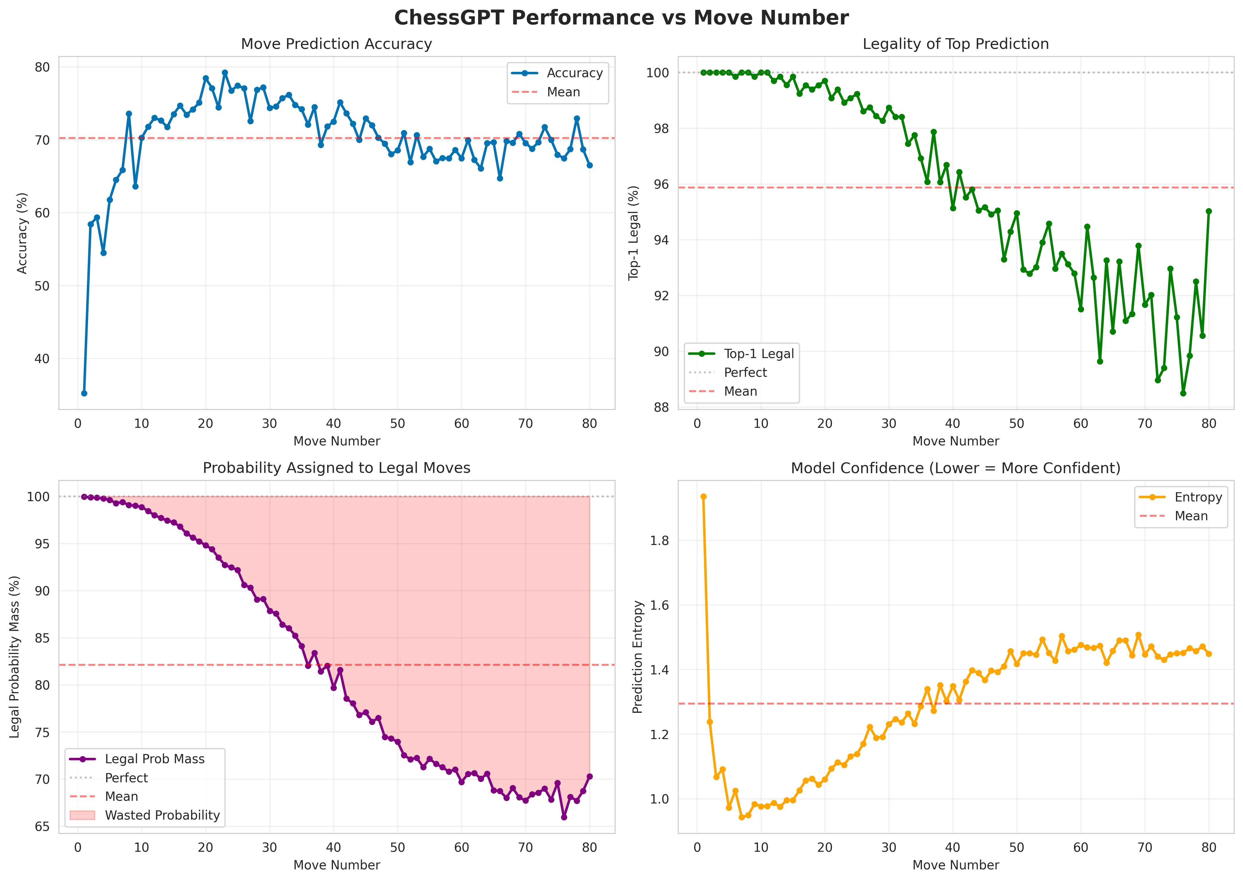
Predicting the exact move a human played is a noisy target, as multiple moves might be equally good in any position, and playing styles vary widely. So I evaluate the model along several dimensions. I was also interested in how these metrics change with respect to the move number in the game. Below are the metrics I evaluated.
Accuracy. What percentage of predicted moves match the moves actually played? This is a strict metric: even if the model's prediction is an excellent move, it counts as wrong if it differs from the game record.
Legality. Perhaps more fundamental than accuracy: is the model even making legal moves? For any board position, the vast majority of possible UCI strings represent illegal moves. There are at most 20 possible starting squares for a side's pieces, and each piece has limited legal destinations depending on its type and the board state. I measure legality two ways:
Top-1 legality: How often is the highest-probability move legal?
Legal probability mass: What fraction of the total probability distribution is assigned to legal moves?
Confidence. How certain is the model in its predictions? A maximally confident model would assign 100% probability to a single move. A minimally confident model would output a uniform distribution. I quantify this using entropy:
H(x) = −Σmᵢ∈M p(mᵢ) log p(mᵢ)
Lower entropy means higher confidence.
results
Performance across various metrics as a function of move number
For all the graphs, note the scales. We see decent accuracy, with rather low accuracy in the opening, highest accuracy during the middlegame, and a plateauing as it reaches the end game. We see very good performance for legality. Notably, where the accuracy is low at the start the the game, the legality is perfect. This makes sense, as there are many openings and it is an ill-posed task to predict what opening someone is going to play. But as the game progresses, the number of good moves to make in a position becomes a much smaller set. In both Top-1 and probability mass, we see a sigmoid-shaped curve with decreasing performance for later moves, but still strong performance overall. Lastly, in terms of confidence, we see validation for the opening, in which the model has very low confidence in its predictions, with entropy decreasing rapidly. Then, as the game progresses, the entropy increases and the model becomes less sure of which move to make.
As an exercise, here's ChessGPT's response to 1. e4, the most common opening move:
rank
move
probability
1
c7c5
25.44%
2
e7e5
24.15%
3
e7e6
17.53%
4
c7c6
9.02%
5
d7d5
6.19%
6
d7d6
5.23%
7
b7b6
3.99%
8
b8c6
3.56%
9
g7g6
2.39%
10
g8f6
1.82%
Top 10 predicted responses to 1. e4
These are all legitimate, commonly-played responses to 1. e4, ordered roughly by popularity in real games. The model has learned the statistical distribution of chess openings.
Then, I played a few games with it. Anecdotally, while it is far from a great chess player, it is not an awful player. It handles openings reasonably well, makes sensible developing moves, and occasionally finds nice tactical ideas like forks. But it also misses obvious opportunities like a free piece sitting in front of a pawn, or an escape via check when under attack.
It plays like someone who has just learned the rules and understands how pieces move, but hasn't yet developed the pattern recognition that makes strong players. This is perhaps unsurprising: the model was trained to predict human moves, not to win games. It has learned the distribution of chess, not the optimization of chess.
[3] probing
While the model is able to perform well, I would like to know what is actually going on. What is the model learning? How is it able to know which moves are legal? To do this, I make use of probes, specifically linear probes. There is an idea called the Linear Representation Hypothesis which proposes that high-level concepts are encoded as simple, straight directions in LLMs' representation space. It has been shown that a similar model trained on Othello learns a linear representation of the board. My goal is to linearly probe for various concepts and help determine what the model is learning.
setup
With a frozen, pretrained model, we pass a data point through, then grab the latent values (aka residual stream) between every layer. We could even go as far as sampling between attention and mlp layers to understand the affects of each, but I treat these as one unit and sample between attention-mlp pairs. Additionally, it may be insightful to train a different probe for even and odd moves, but for simplicity (and compute) I opt to train one probe per layer per concept across all moves.
For each data point we pass through, we know some ground truth that is not immediately obvious upon looking at a sequence of moves. For example, an easy property is whose move it is: black or white. We construct a dataset across many games which consists of the moves as input and the ground truth property as the label. Then, we run the model and train a linear probe on each layer that takes in the residual stream at that layer and predicts the ground truth property.
The properties I decided to test were:
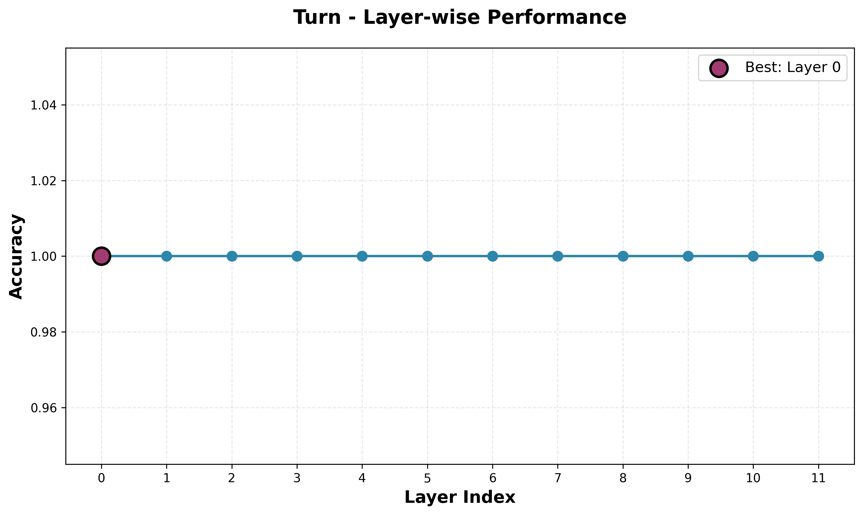
Turn. A binary classifier that predicts whose turn it is. The simplest probe, and because of the high legal move rate, I expect very good performance on this.
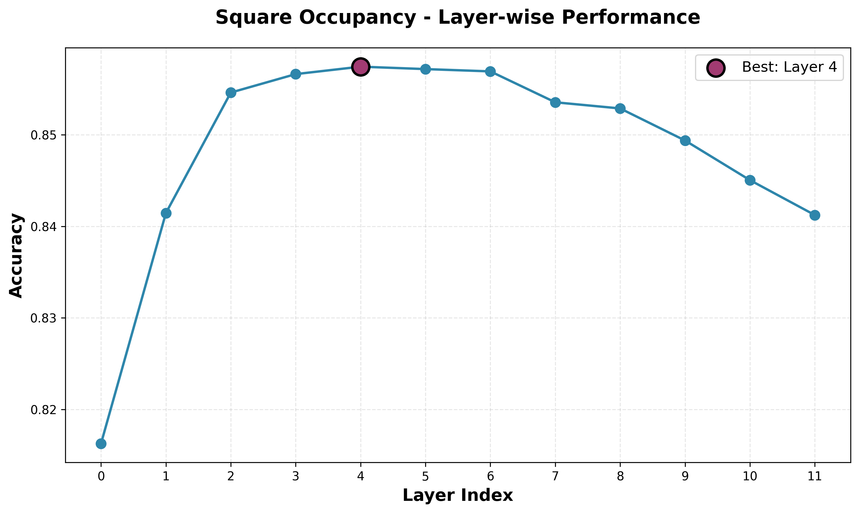
Square Occupancy. For each of the 64 squares, I train a separate probe that predicts if that square is occupied. This is a simplified board state probe.
Piece Location. Here, I ask where each piece is located. For all 12 piece types (6 white and 6 black), an independent multi-label binary classifier predicts a 64-dimensional binary vector that indicates which squares that piece occupies.
Material. There are two probe types here. First, I have 12 probes, one for each piece, that predict the count of that piece. Then, I have one probe that predicts the material balance (in pawn units). These are all ridge regressors. I am unsure on performance here, as material balance is not necessarily the best representation of the game.
Positional Rules. These probes test hidden game state features not visible on the board. There are five binary classifiers for white can castle kingside, white can castle queenside, black can castle kingside, black can castle queenside, and en passant available.
Board State. In addition to the square and piece probes, I wanted a granular board state reconstruction system. I train one binary classifier for each piece for each square, giving 832 (8 × 8 × 13) probes per layer. In hindsight, this may have been overkill and took a long time to train, but it is definitely comprehensive and gives us a nice peak into the model's view of the board.
Tactical. For a series of tactical puzzle themes (fork, pin, skewer, etc), I train a classifier. For this, I used puzzles from the Lichess puzzle dataset. Each datapoint has a set of theme associated with it, giving us some ground truth, even if the length of the puzzles differ. This dataset is positional, meaning it doesn't have the moves, so I grabbed the gameID from each puzzle and used the Lichess API to get the moves from each game up to the puzzle start. Also, while other concepts here were important for playing legal moves, this is not necessarily true here, and tactics are quite high level, so these results will be interesting.
probing results — turn probe
Turn probe accuracy across layers
To no surprise, the turn probe has perfect accuracy across all layers. Given the model's ability to predict legal moves, it must know whose turn it is, and pretty much any decisions about what the next move is going to be depend on who is moving. It would be interesting to see how the model is predicting this, as it could be taking some modulo of the number of moves so far, memorizing that even moves and odd moves correspond to black and white (one indexed), or even using the previous move to deduce who just moved.
probing results — square occupancy probe
Square occupancy probe accuracy across layers
We see strongest square occupancy performance from layer four, with decent, but far from perfect accuracy. Interestingly, the accuracy is lower for the first few layers, before peaking at layer four then steadily dropping. We expected to see lower-level concepts have stronger representations in earlier layers and high-level concepts represented in later layers. Quantifying the "high-levelness" of a concept is a far from exact science, but we can take a rough, intuitive guess for each of our concepts. For turn, this is obviously very low-level. For square occupancy, this is not extremely low-level, but still relatively simple compared to the concepts required to play chess.
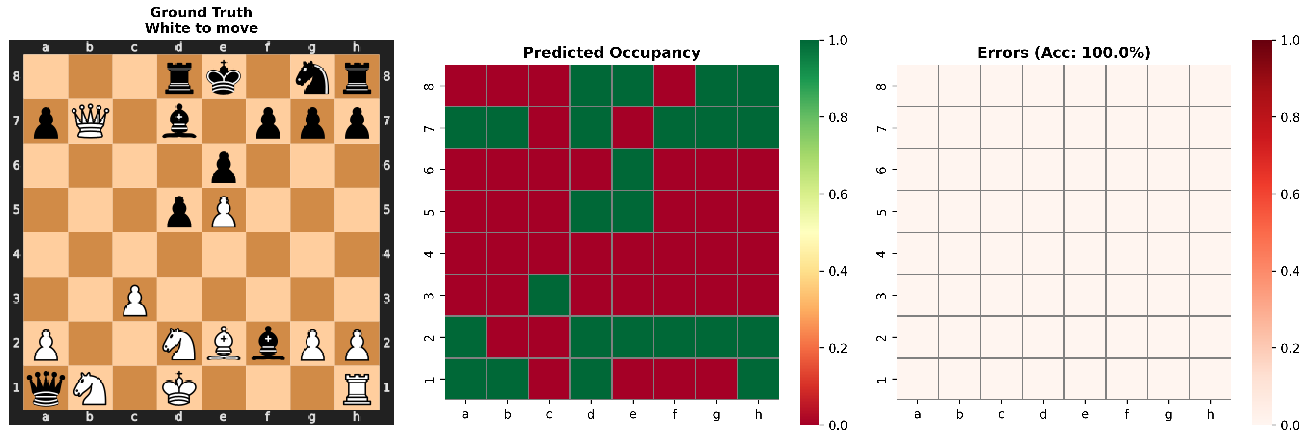
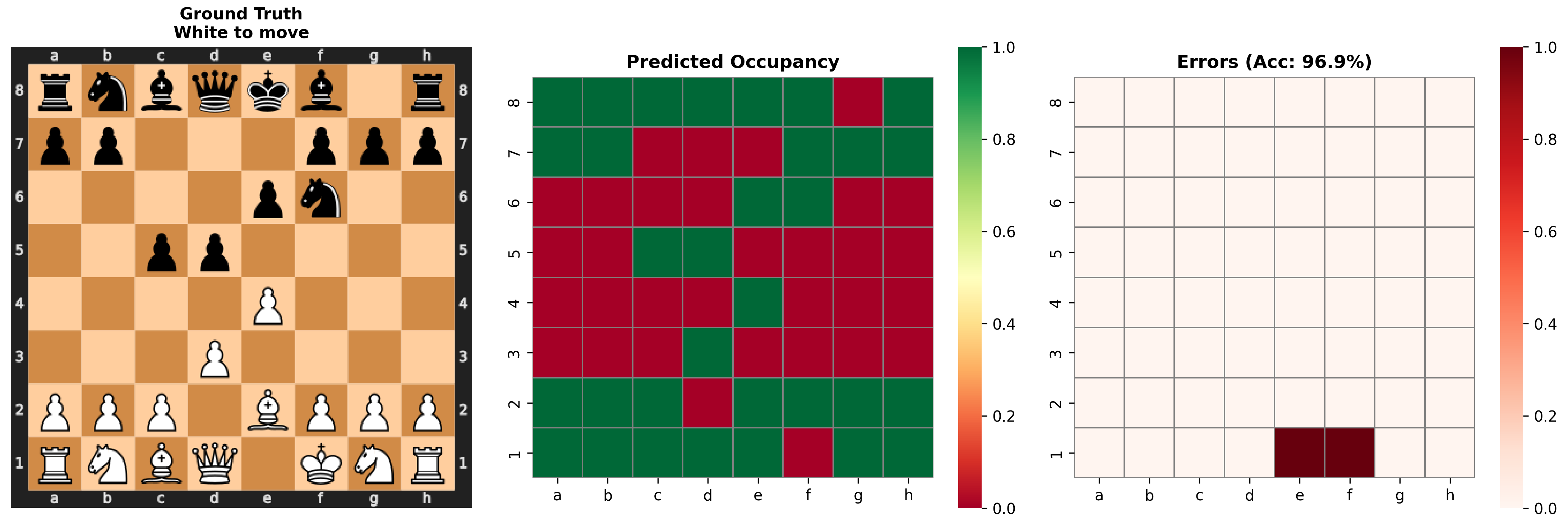
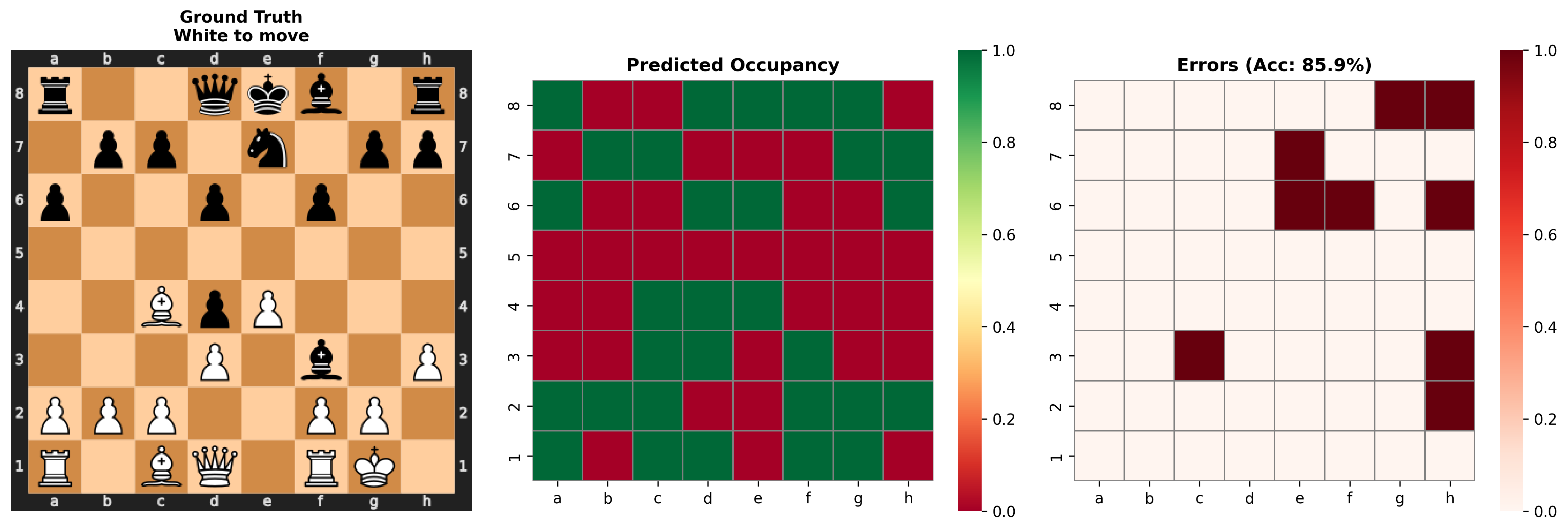
Occupancy Example 1Occupancy Example 2Occupancy Example 3
Examining some specific cases when probing layer 4, we see the model has a strong understanding of square occupancy even in complicated cases. In one position, the opening looks standard, except white's king is moved from its home on e1 to f1. The model misses this, thinking e1 is occupied and f1 is open. This suggests that while the model is strong in common positions, it breaks down in strange positions. This poor out-of-sample performance was an original issue with AlphaGo, and is attributed to its loss in the 4th game against Lee Sedol.
probing results — piece location probe
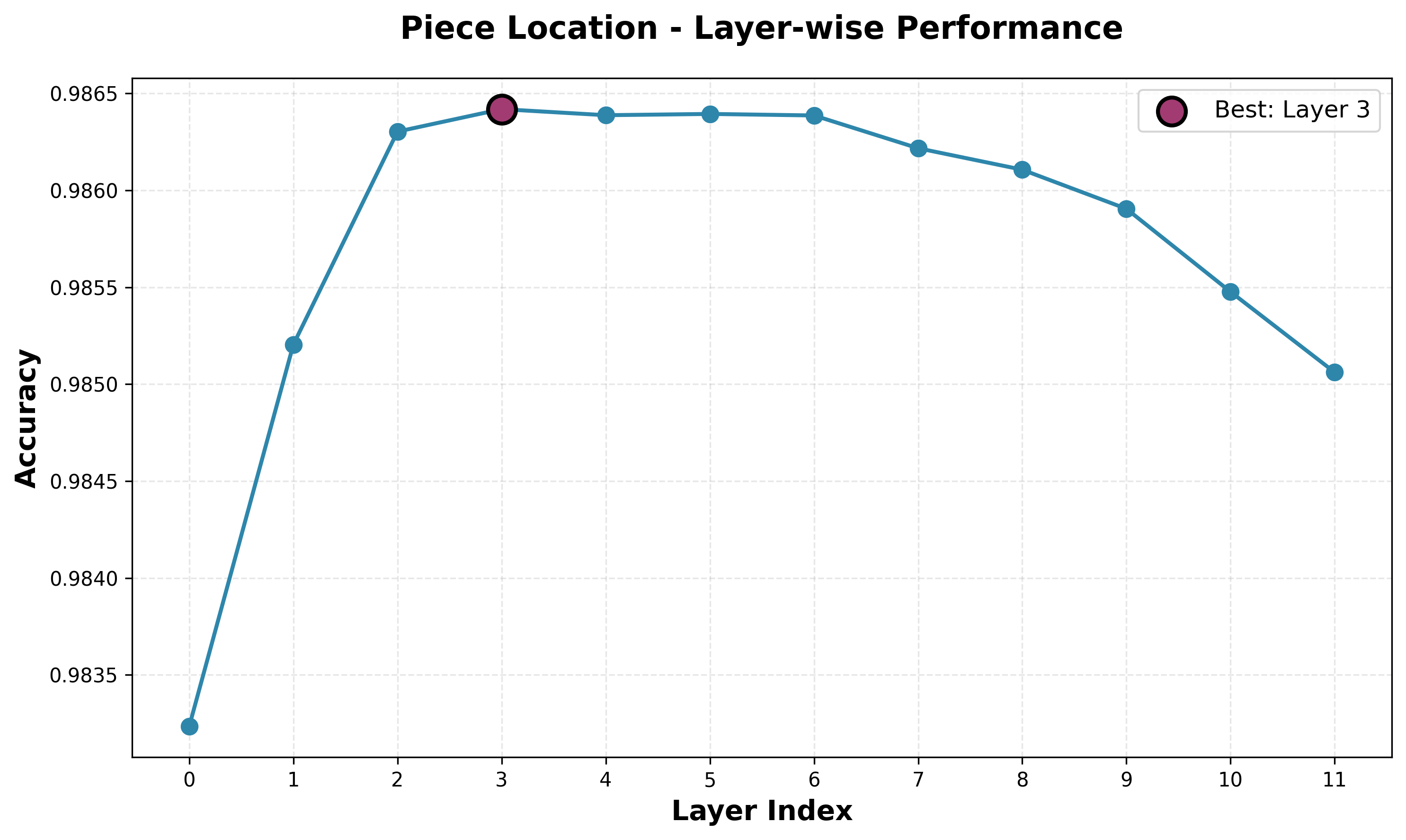
Piece location probe accuracy across layers
Our piece location probe has incredibly high accuracy. Note accuracy scale: the difference between the best and worst performing layers is only 0.003. Still, despite the scale we see a clear pattern emerge, with best performance at the early middle layers and a slowly decreasing performance with later layers. It is an almost identical curve to the square occupancy curve. The high performance suggests the piece location is very important to the model, which makes sense. The performance over the simpler square occupancy tasks also suggests that the model is storing information in a manner similar to this task. Sensibly, piece-level information is much more useful than square occupancy.
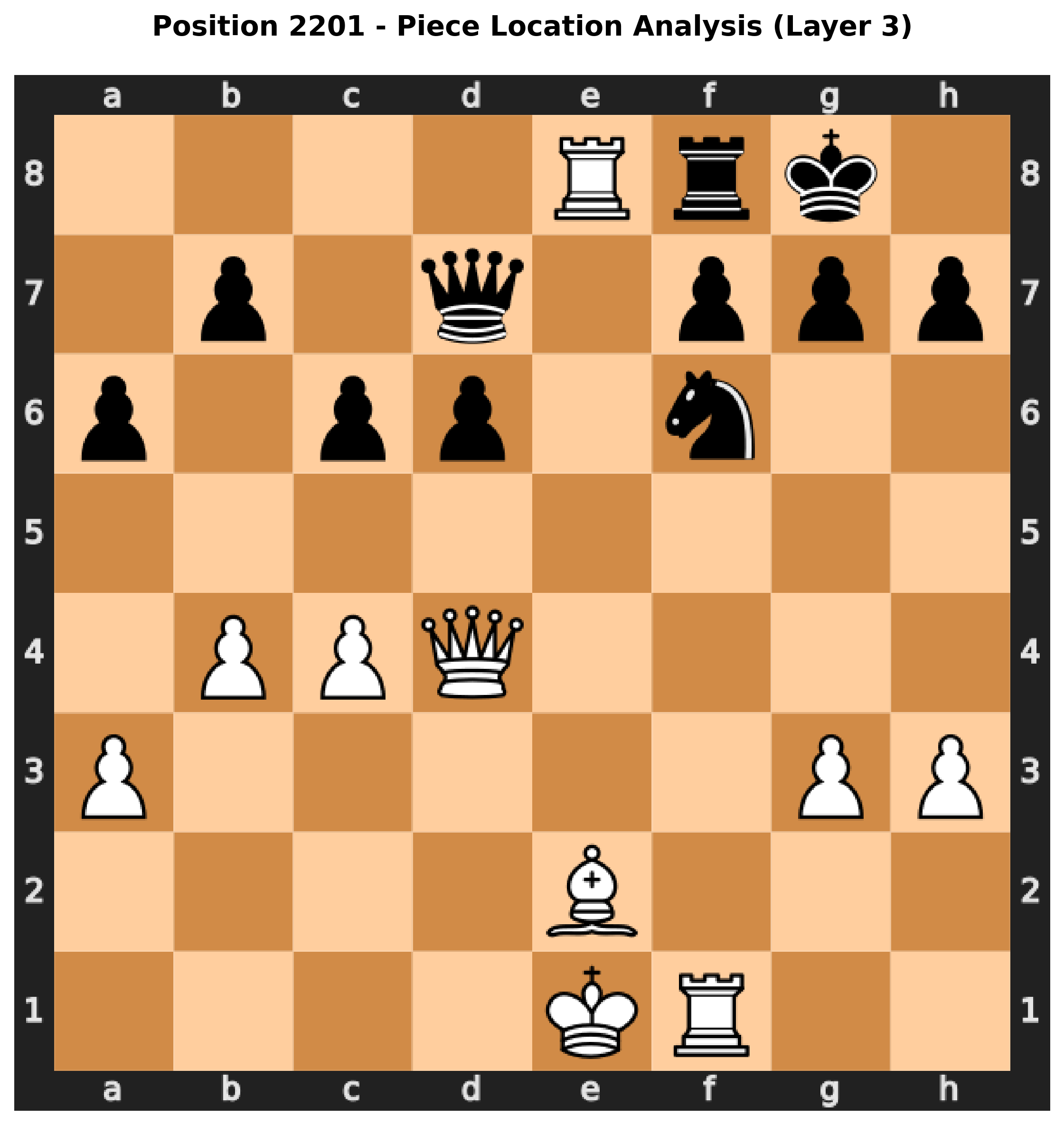
Piece location predictions for a sample positionHeatmaps showing piece location predictions by piece type
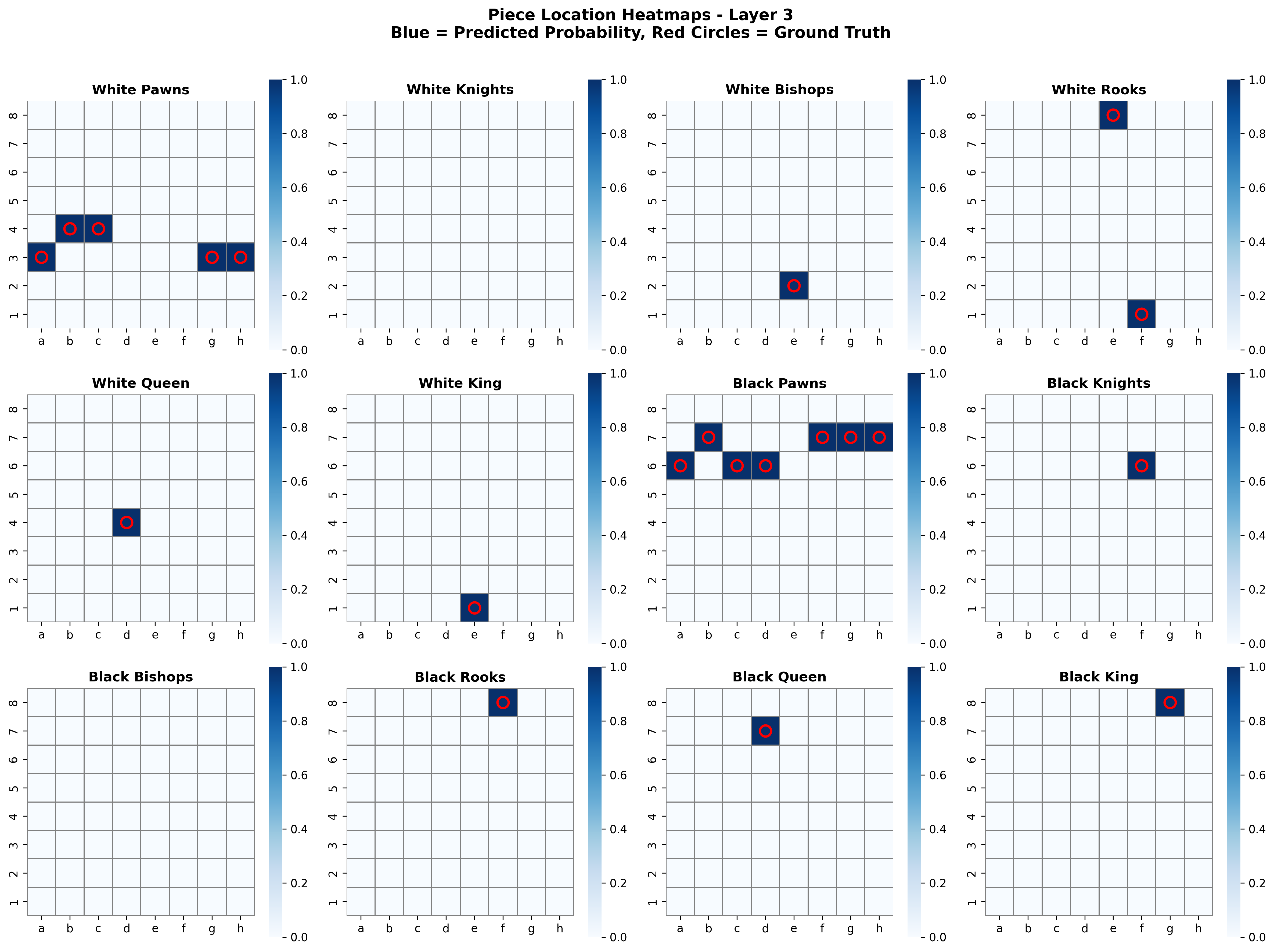
Here we see the predictions of the piece locator probes for a random position. While this position is not complicated, it is not simple, but the model is able to predict the exact locations for each piece type, including predicting the right number of pawns, only one location for pairs that have lost a piece, and no locations for piece types completely captured.
probing results — material probe
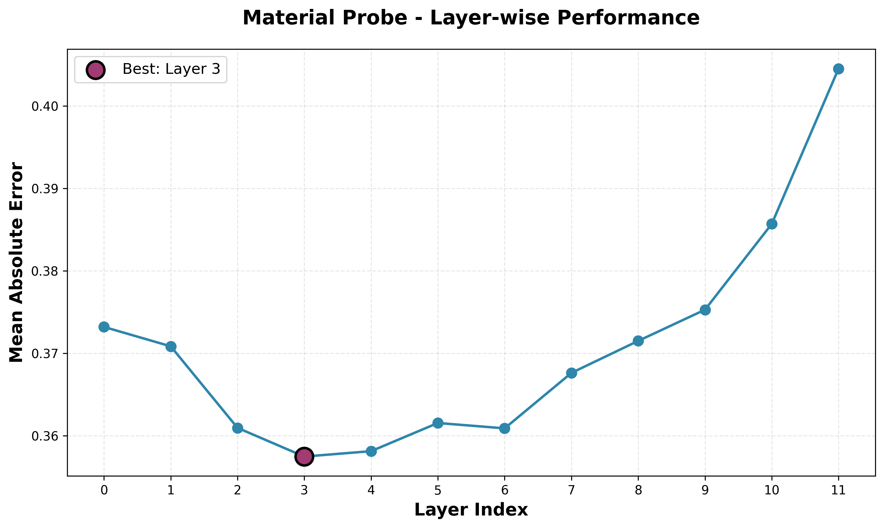
Material probe mean absolute error across layers
Here, I am graphing the mean absolute error (MAE) in predicted material difference and actual material difference, so lower is better. We again see the same trend as the piece location and square occupancy curves, which makes sense, as the material difference is simplified version of the piece location task. The MAE is also quite low, which is sound given the accuracy of the piece prediction probe.
probing results — positional rules probe
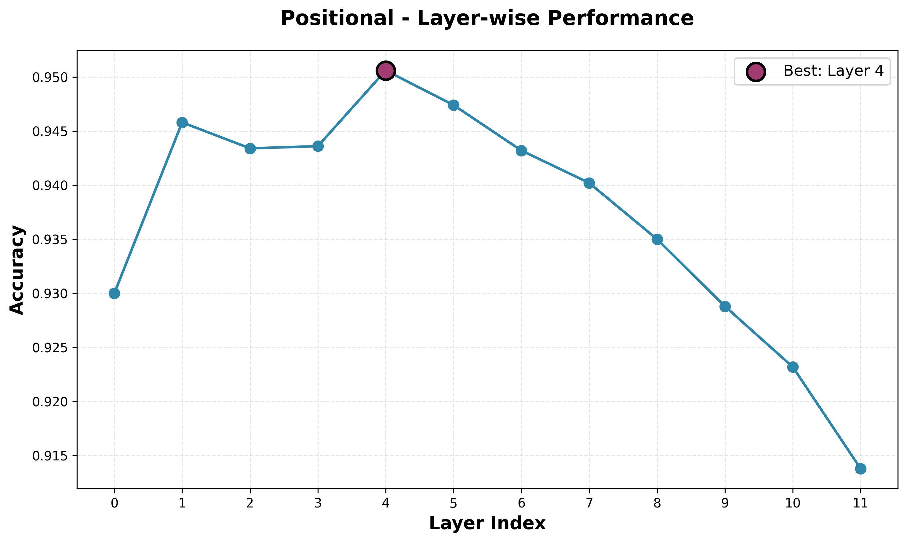
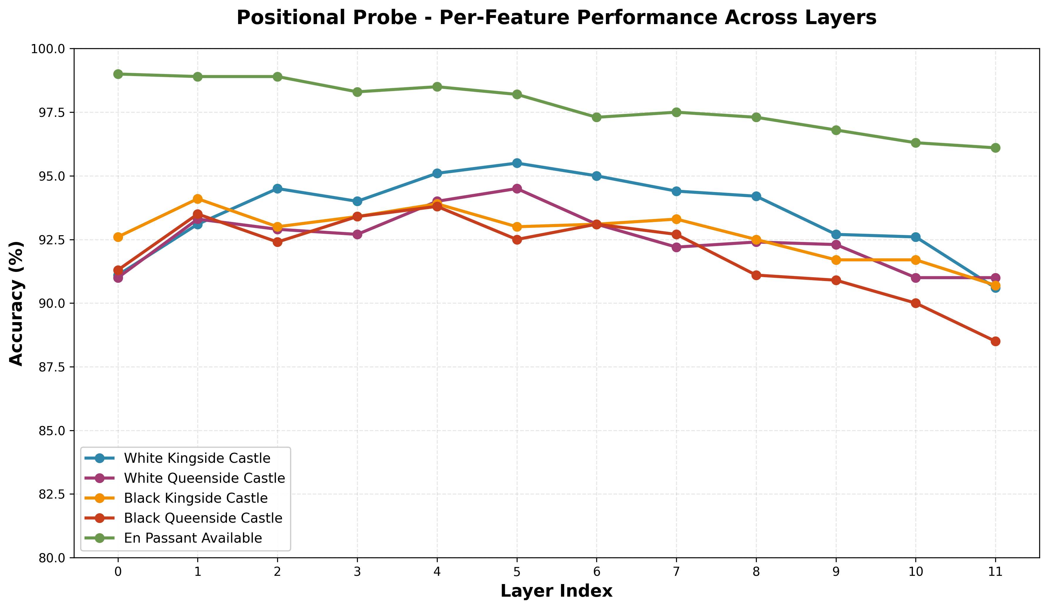
Positional rules probe accuracy across layersAccuracy breakdown by positional feature (castling rights, en passant)
The model has decent understanding of hidden positional rules. While the average performance peaks in layer 4, we see this is not necessarily the best layer for each of the individual features. En Passant has a near monotonic decrease in performance after layer 0. The castle performances are all similar, though comparing side performances (kingside vs queenside) for white and black, we see a constant stronger performance for white, and within white and black we see a constant better performance for kingside over queenside.
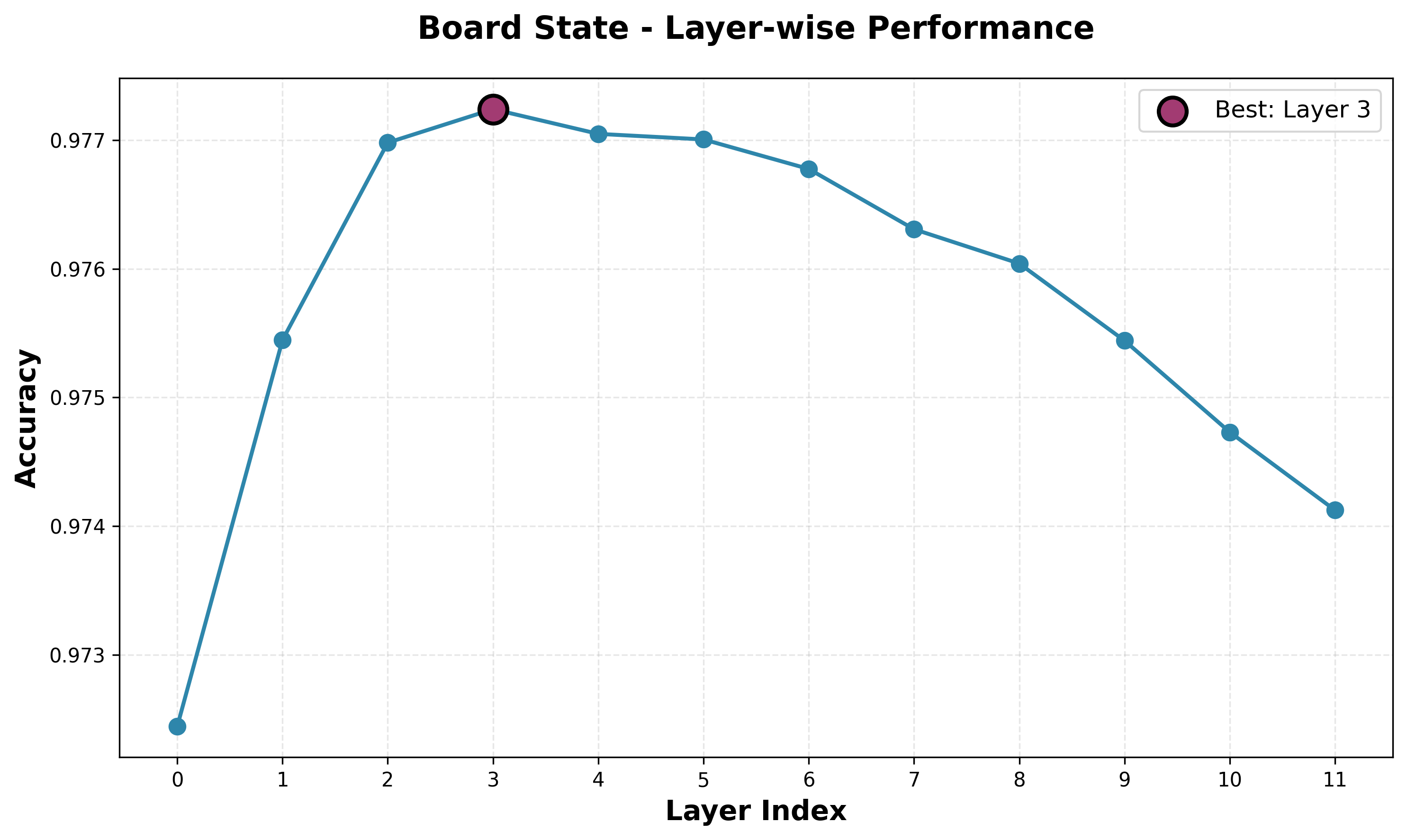
probing results — board state probe
Board state probe accuracy across layers
The board state probe shows the same shape and similar performance to the piece position probe. This is just another way of trying to capture the same state, so it is validating to see that they both have similar performance.
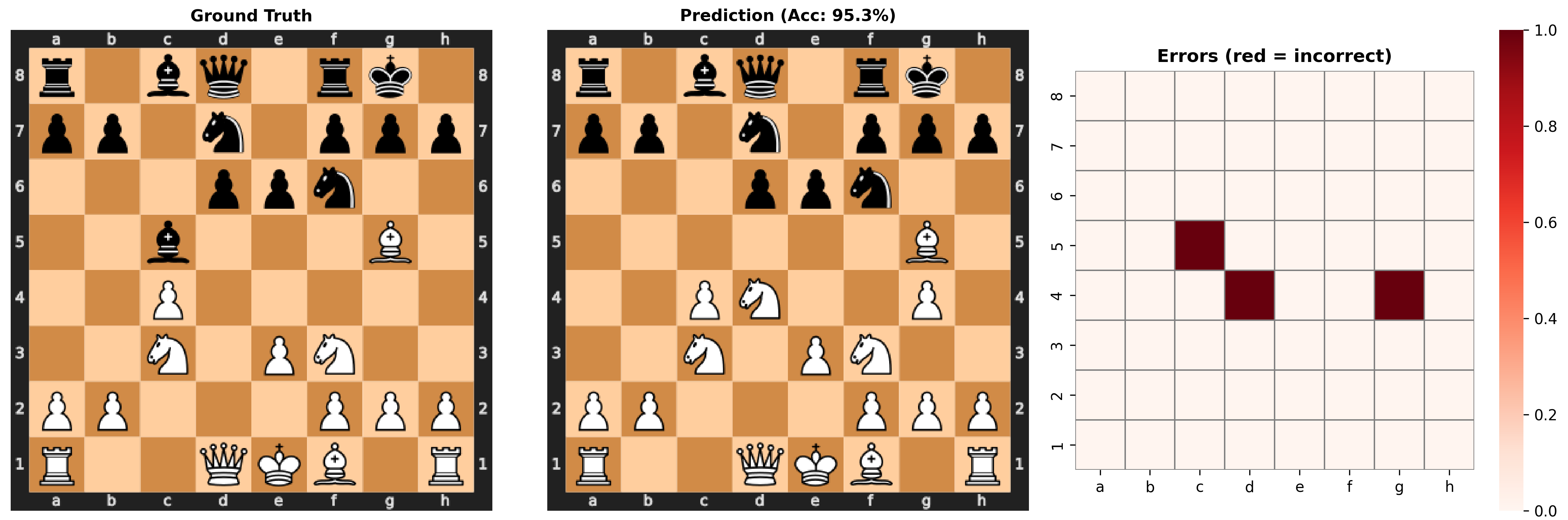
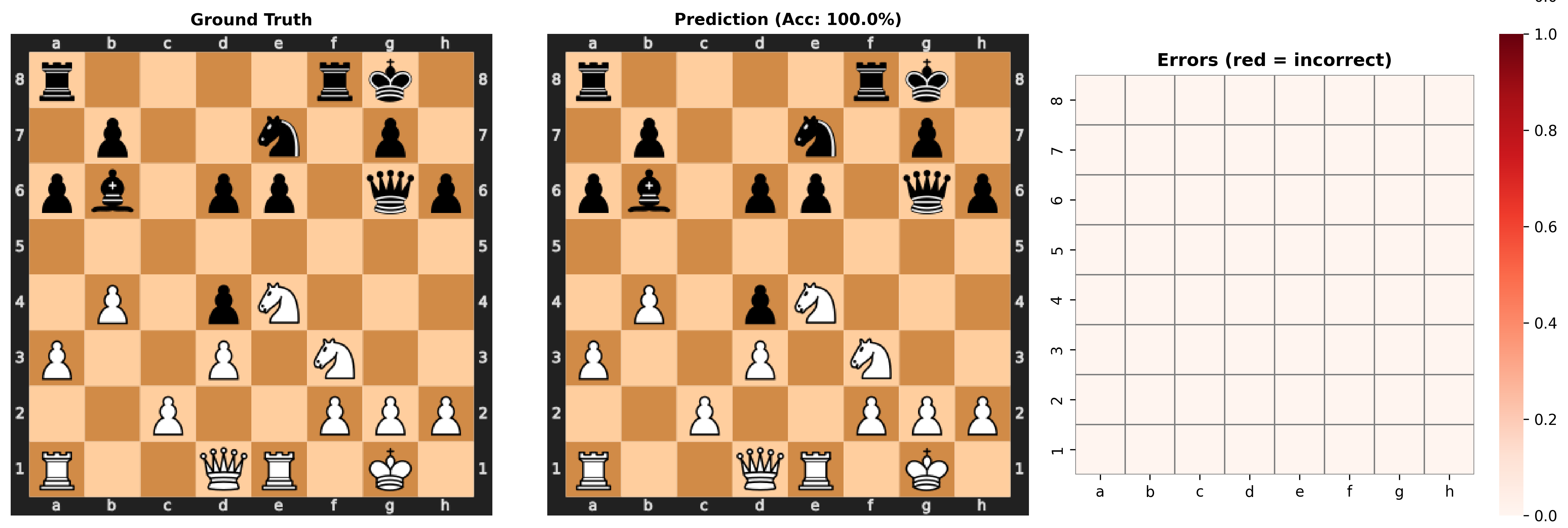
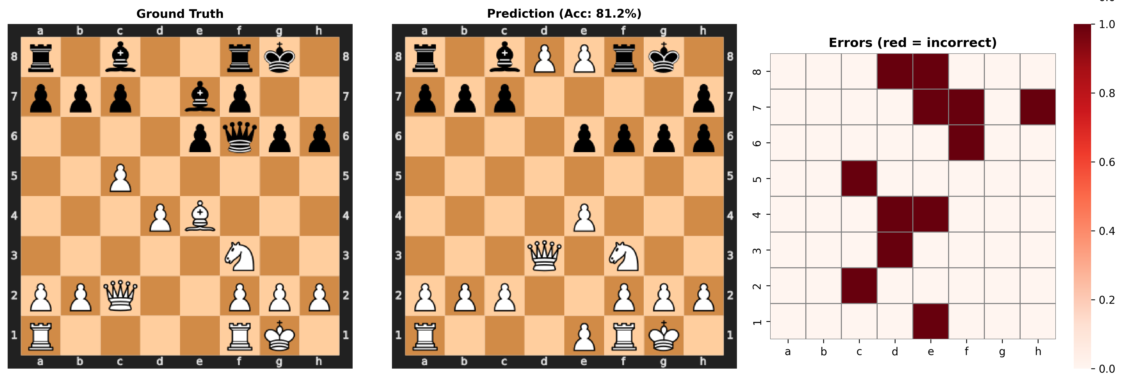
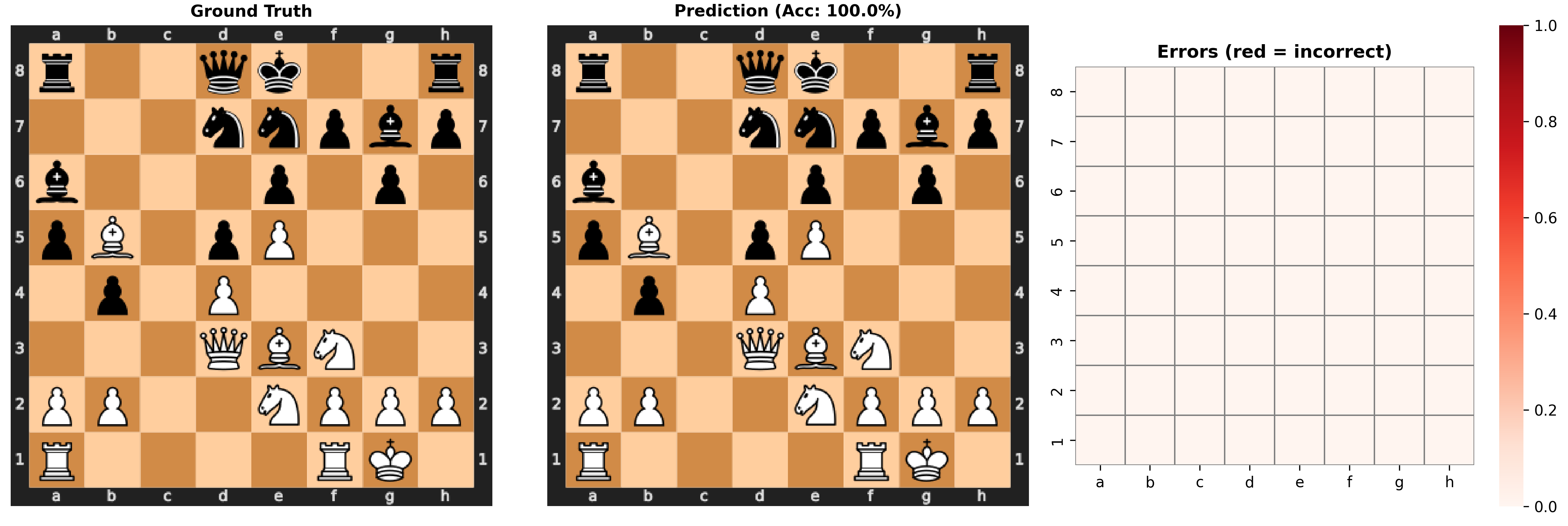
Reconstruction Example 1Reconstruction Example 2Reconstruction Example 3Reconstruction Example 4
Looking at some random positions, we can see that most of the time it does a perfect job reconstructing the position. Occasionally, it will make small errors, some of which are nonsensical like three knights. Sometimes, however, it fails a lot of the pieces, even though it still gets a decent accuracy. It seems in these catastrophic failures, it fails in nearly every way: it misses some pieces, it moves some pieces, and it replaces a bunch of pieces with pawns, including white pawns on the eight rank and the first rank! This suggests that in these cases it is not just one probe or one small part of the representation that is insufficient, but a large part of the representation that contains the information about many locations and pieces.
probing results — tactical probe
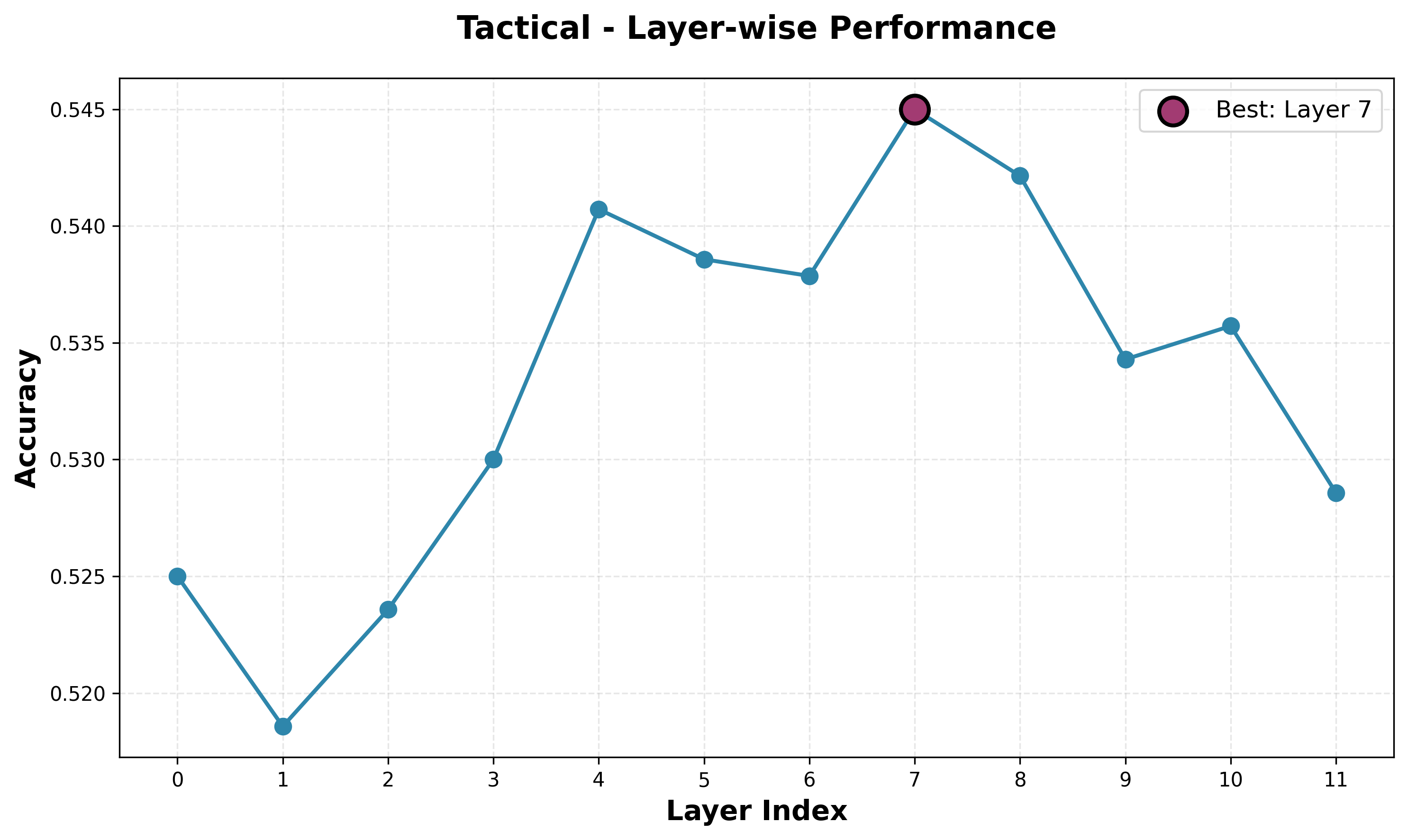
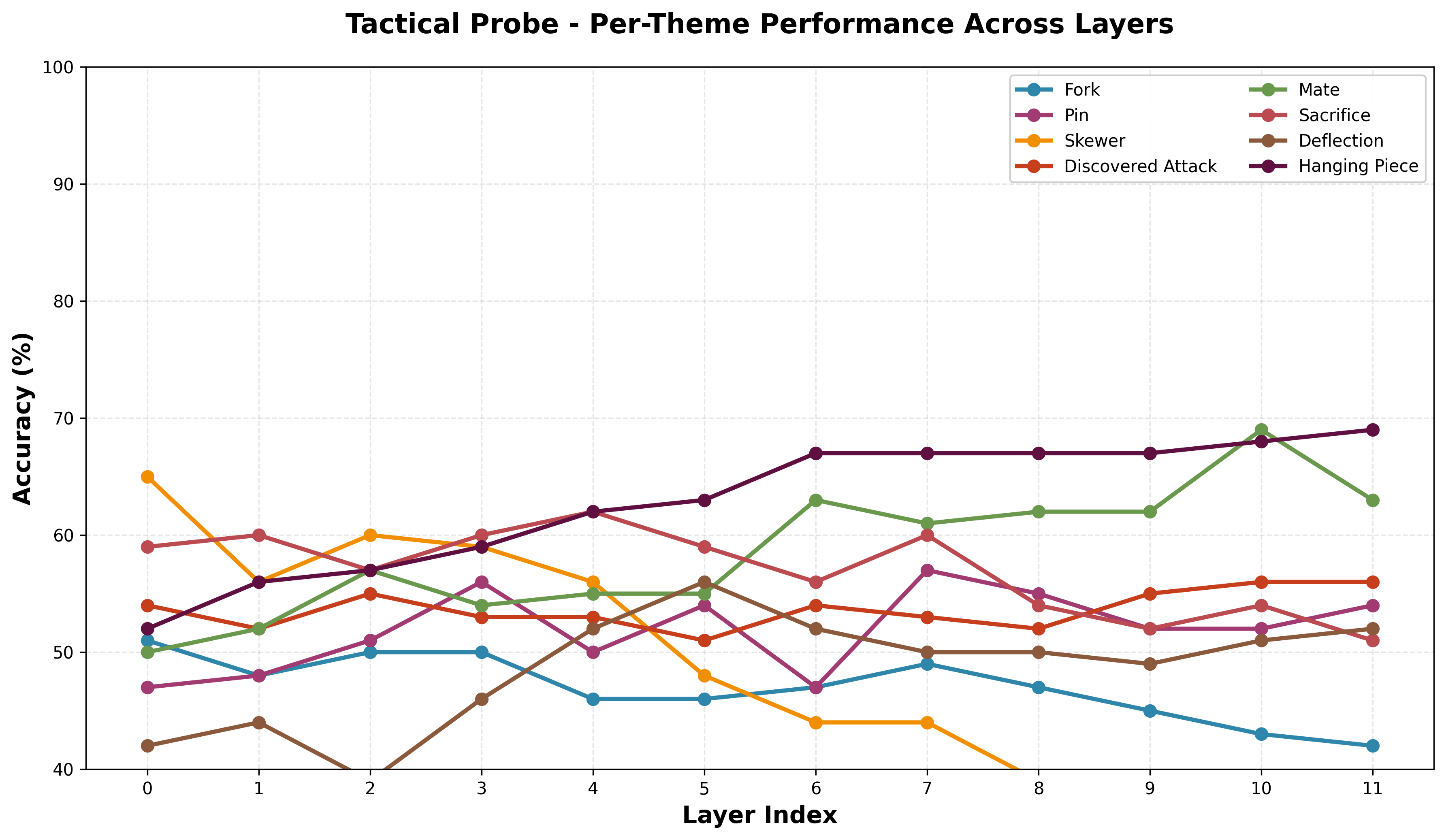
Tactical probe accuracy across layersAccuracy breakdown by tactical theme (fork, pin, skewer, etc.)
The tactical probes have pretty bad performance and lower performance than I had hoped for. At some point across the layers, each model has above 50% accuracy, meaning it is learning something, but not enough to be significant. In part, I think this can be attributed to the smaller model size, and I will probably try to train a larger model with more data and reevaluate performance. We do, however, see a peak in average performance on a later layer, which fits the narrative that higher-order concepts are strongest represented later in the network. Looking at the per-theme performance, it is important to note that performance looks less smooth and more stochastic across layers compared to other probes, though there is a general upward trend. Different patterns have relatively clearly stronger representations at different points in the network, but it is hard to make a definitive claim about higher or lower order patterns being represented well at different points.
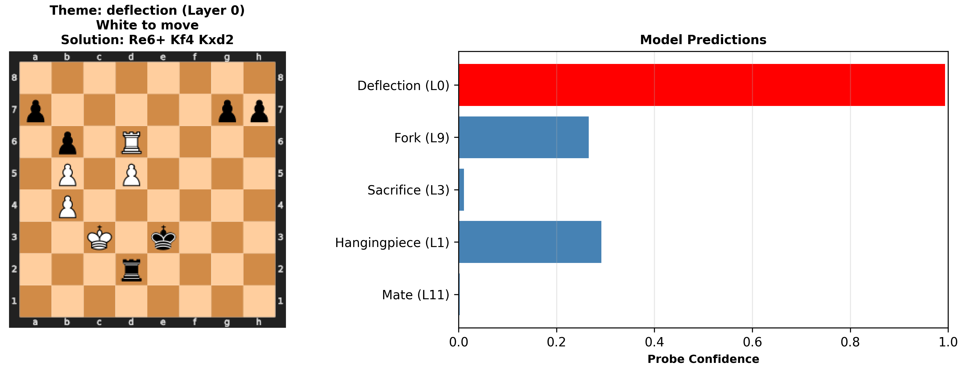
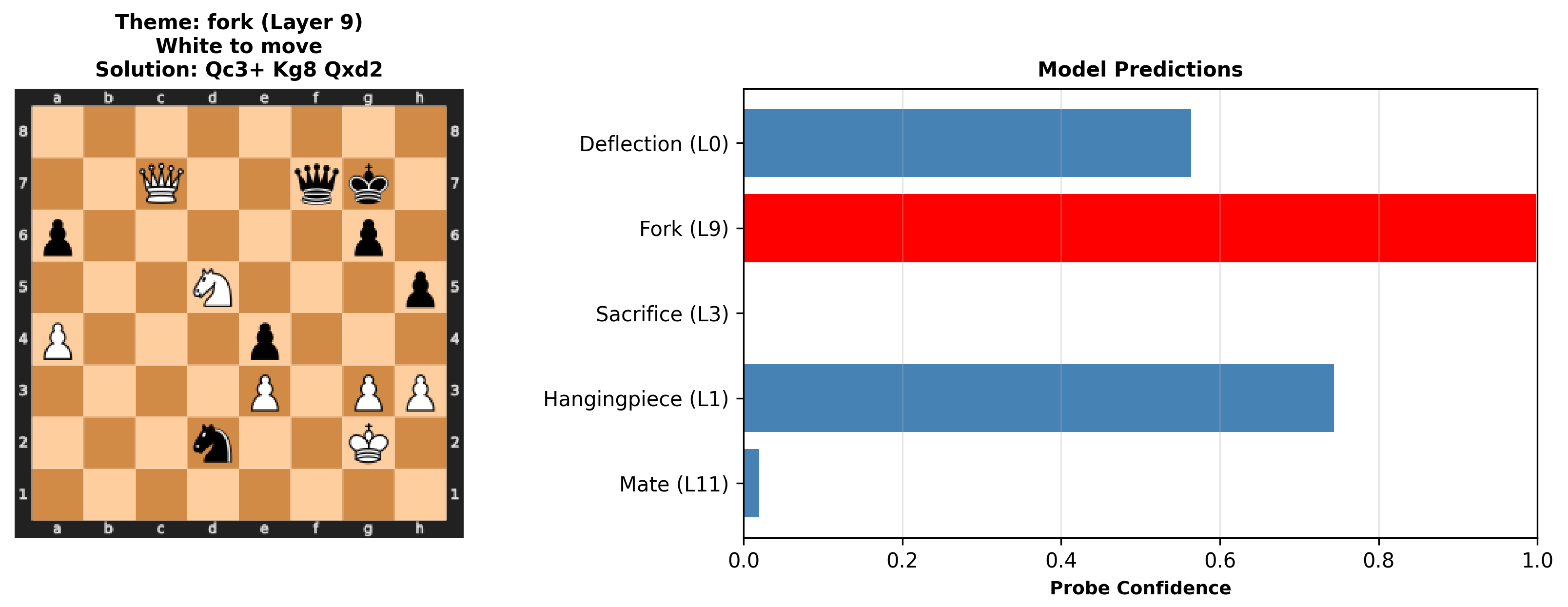
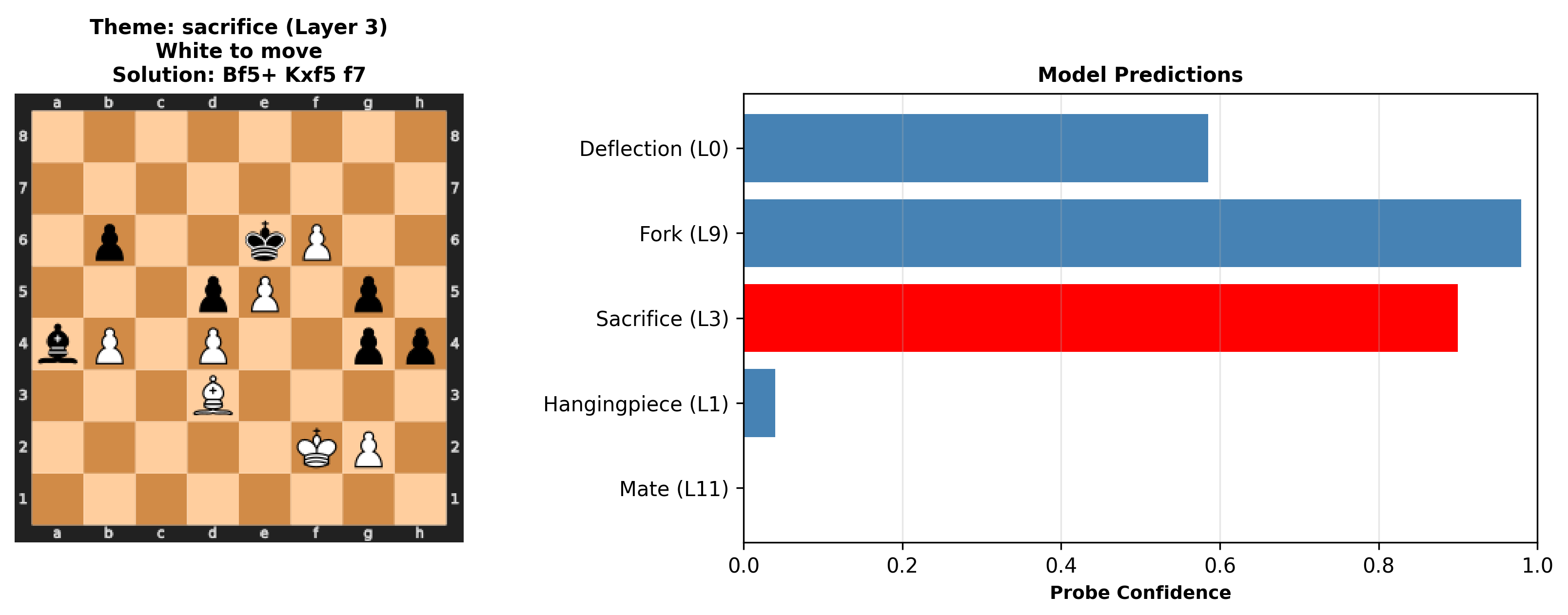
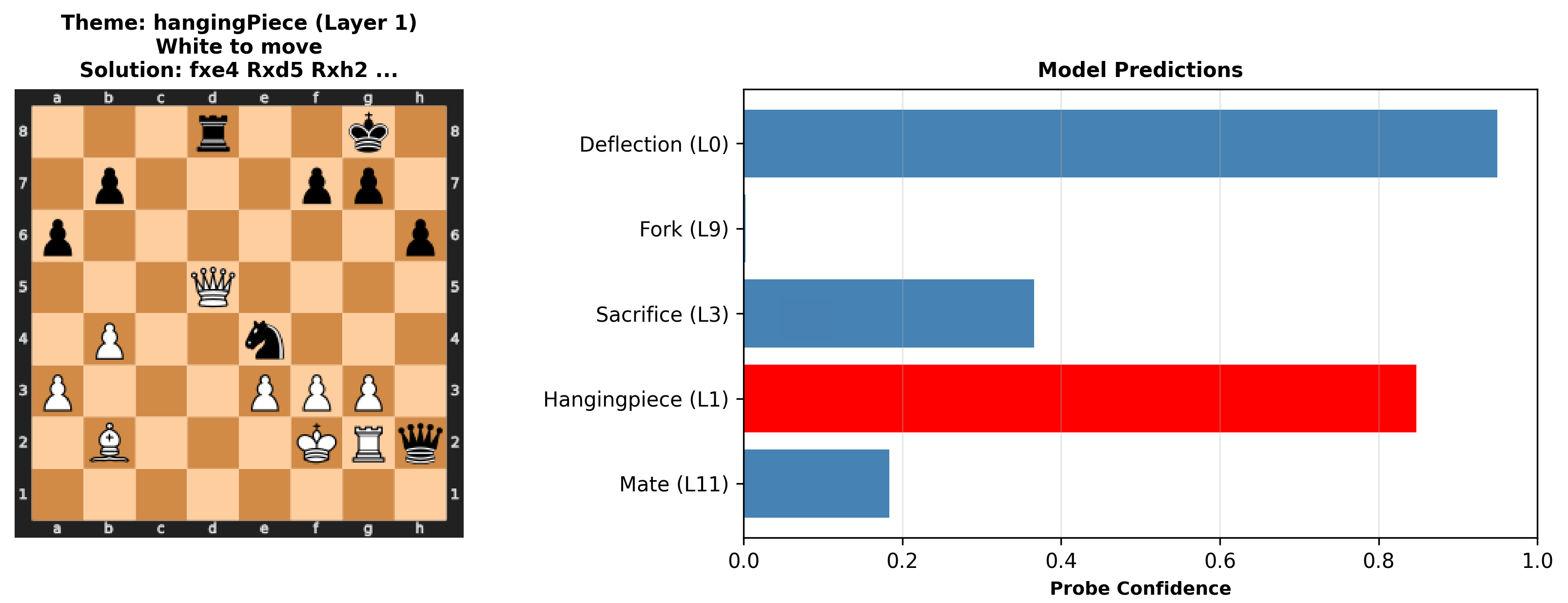
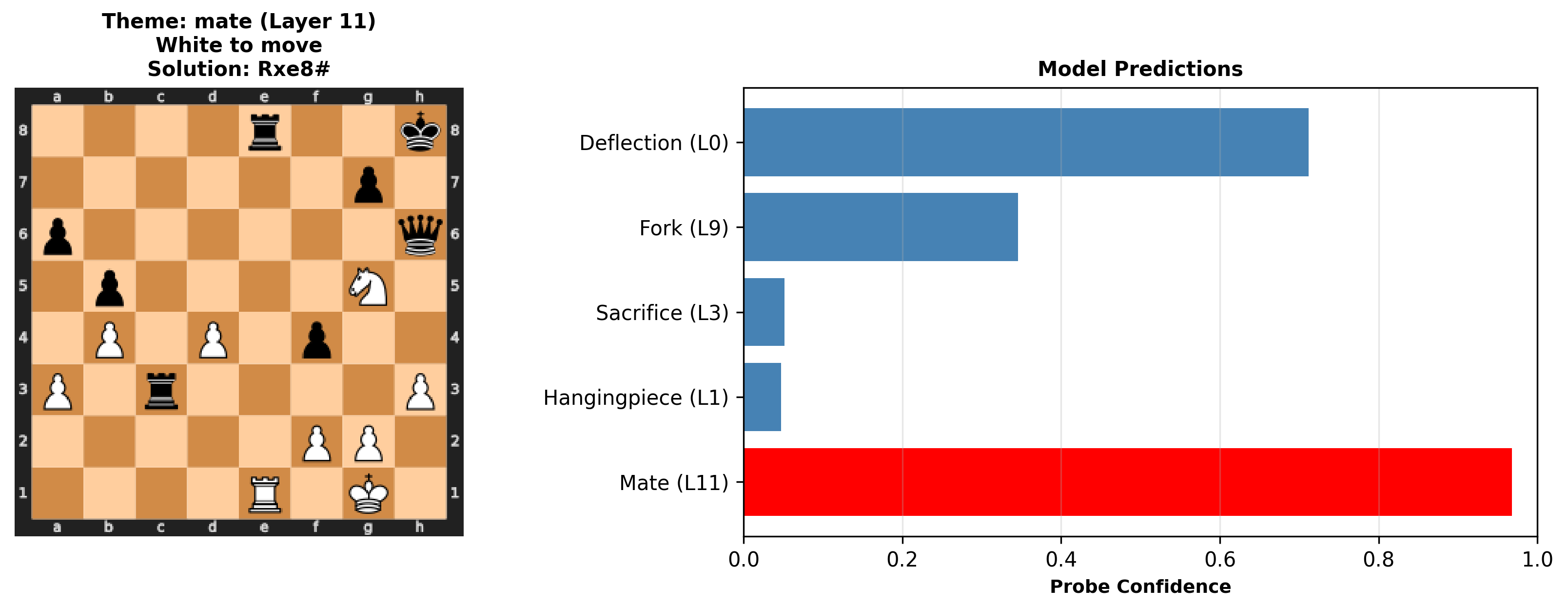
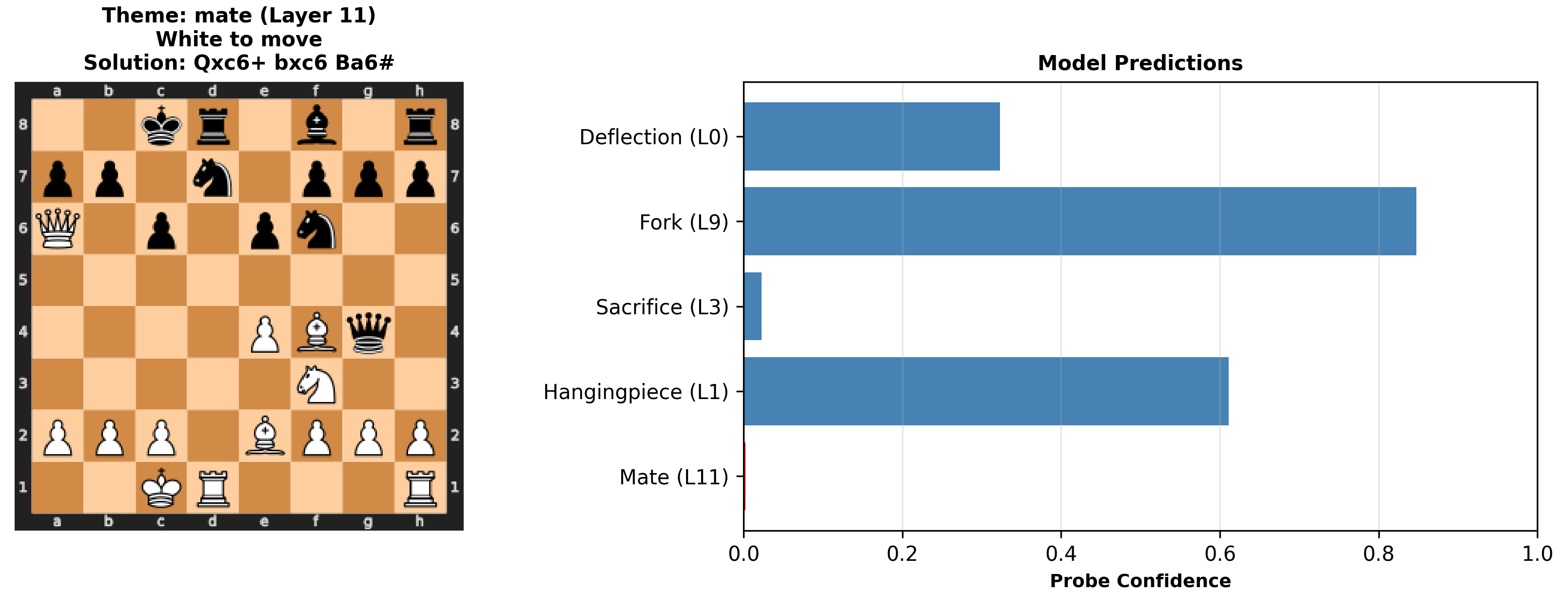
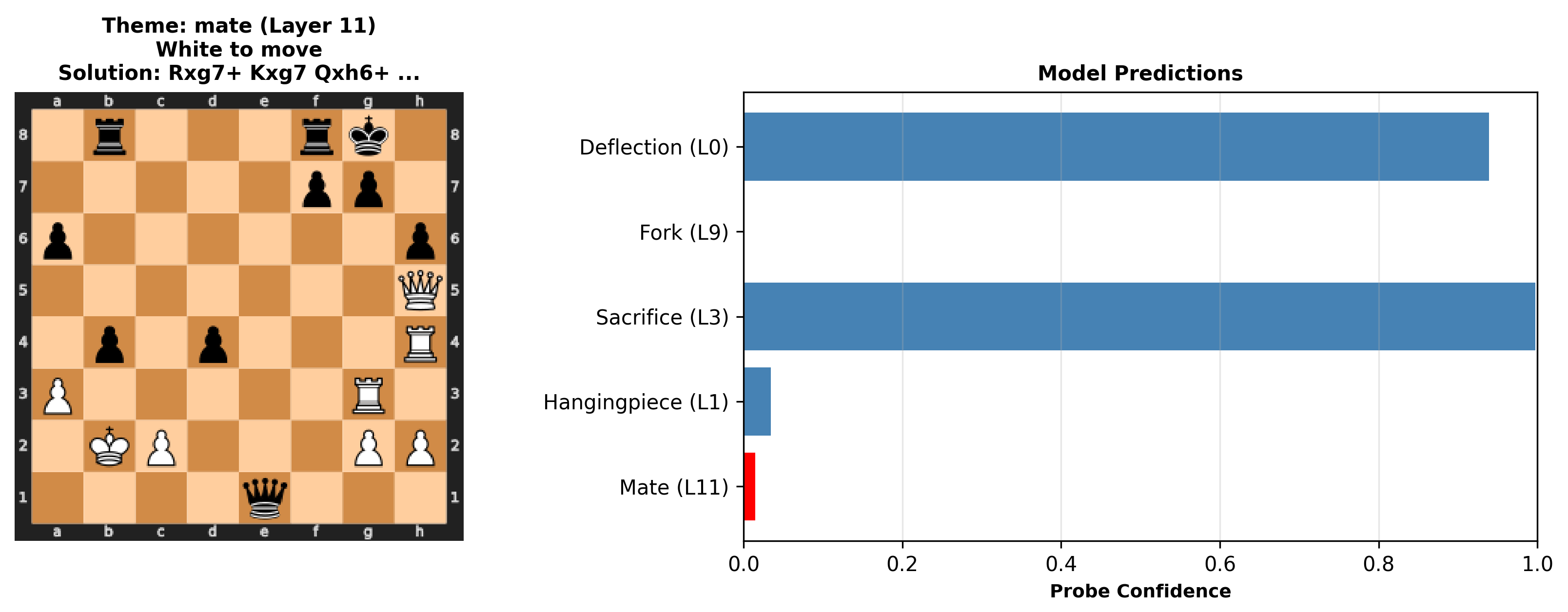
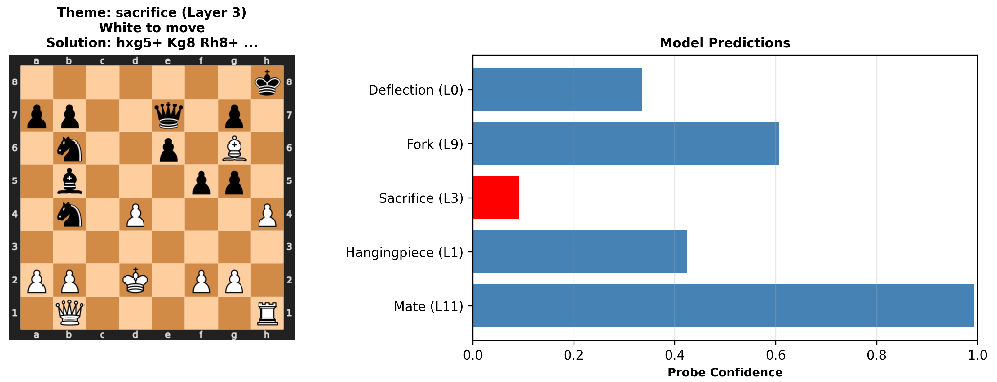
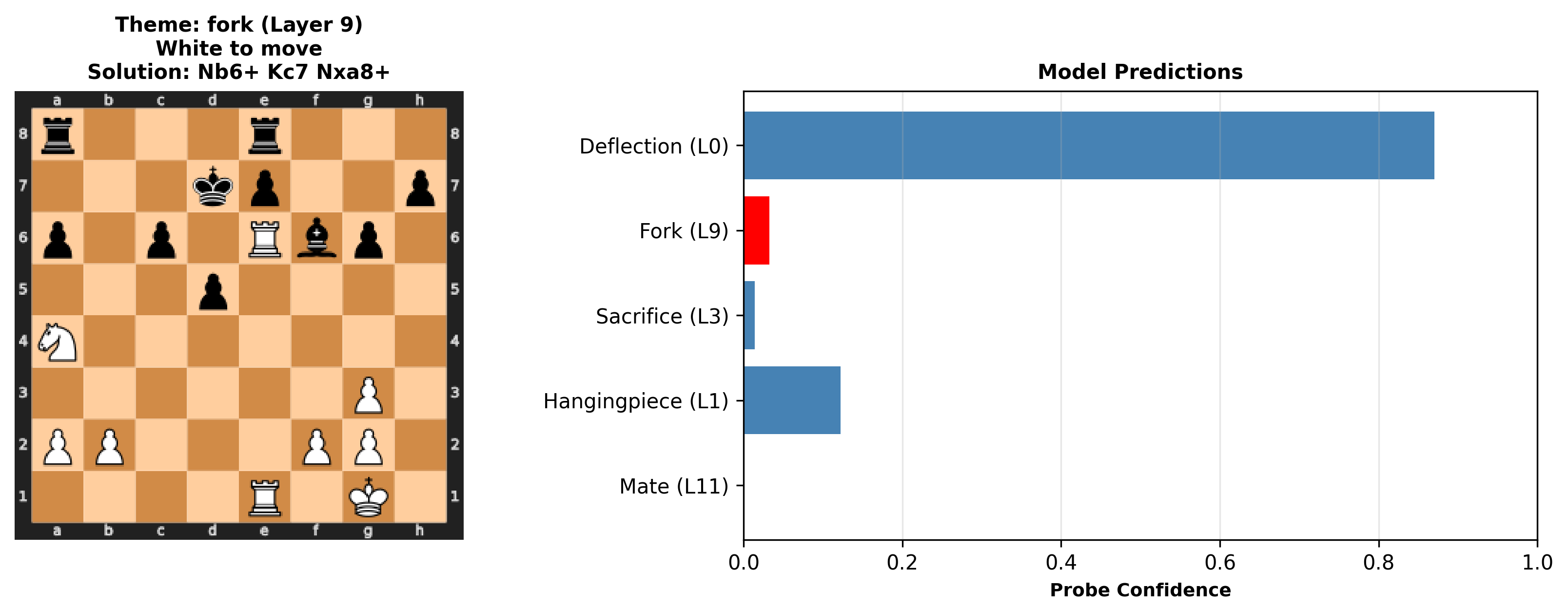
Tactical Example 1Tactical Example 2Tactical Example 3Tactical Example 4Tactical Example 5Tactical Example 6Tactical Example 7Tactical Example 8Tactical Example 9
Looking at some examples, we see the model does very well on obvious puzzles, and is even able to discern some more complicated tactics. Note that some puzzles have multiple themes, and while I only display one theme in the title, these themes are correctly used when training and evaluating. However, when a theme is not present we still see some probes detecting tactics. Moreover, the model just completely fails to detect the theme in some puzzles. This seems especially to be the case with longer puzzles, and it may be worth trying to limit the dataset to only a few moves, or even training a different probe for different look ahead distances. Still, I would hope to see the feature for a given tactic present in advance of the given state that has that tactic, as this would show the model has some understanding of not just the game now, but where the game is heading and what moves will be available then.
For a future direction, I would like to test the model's puzzle performance, seeing which moves it takes. I suspect that even though it is identifying themes, it may not be able to actually find the right sequence of moves. I think overall, scaling up training, including model size, data, and train time, may give clearer features, especially for tactics.
Ferromagnetism and phase transitions are fundamental concepts in statistical mechanics. The Ising Model provides a simplified yet effective framework to study these phenomena by modeling spins on a lattice. This report focuses on a 3D Ising Model and its application to high-dimensional problems.
The Ising model, first proposed by Wilhelm Lenz in 1920 and solved by his student Ernst Ising in 1D, has become one of the most important models in statistical physics. It successfully describes ferromagnetic-paramagnetic phase transitions and serves as a paradigm for understanding critical phenomena.
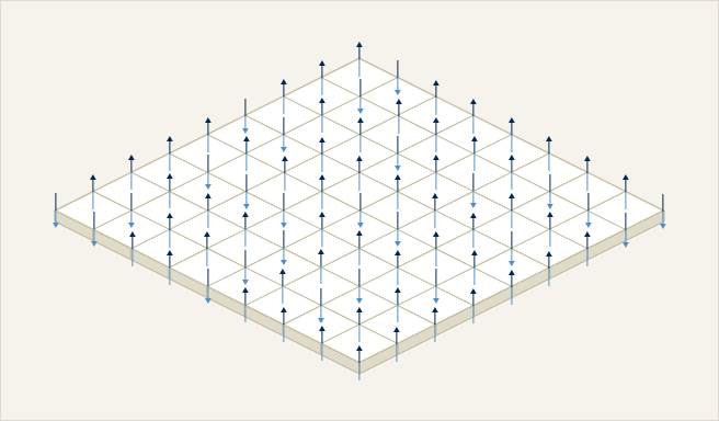
Ising model example
In ferromagnetic materials, atomic spins tend to align parallel to each other below a critical temperature (Curie temperature), resulting in spontaneous magnetization. Above this temperature, thermal fluctuations overcome the alignment tendency, leading to a paramagnetic phase. The 3D Ising model captures this behavior through nearest-neighbor interactions on a cubic lattice.
Objective
The goal of this project is to simulate the 3D Ising Model using parallel computing approaches, leveraging MPI for distributed memory and GPUs for acceleration. Special emphasis is placed on scalability, performance optimization, and future enhancements. I aim to:
Implement and analyze the 3D Ising model below its critical temperature
Study finite-size scaling effects in large systems
Develop efficient parallel algorithms for spin updates and energy calculations
Compare different optimization strategies for high-performance computing
[2] theoretical background
Ising Model Formulation
The Ising Model represents spins on a lattice, each taking a value of +1 or -1. From physics, I know that the system will minimize the Hamiltonian. The Hamiltonian is defined as:
H = −J Σ⟨i,j⟩ sᵢ sⱼ − h Σi sᵢ
where J is the interaction strength, h is the external magnetic field, and s_i denotes the spin at site i. The notation ⟨i,j⟩ indicates summation over nearest neighbors only. In my 3D implementation, each lattice site has six nearest neighbors (±x, ±y, ±z directions).
The energy change for a single spin flip is given by:
ΔEᵢ = −sᵢ(J Σneighbors sₙ + h)
where the sum runs over nearest neighbors of site i. This local energy change ΔE is crucial for the Metropolis algorithm implementation.
Monte Carlo Simulation
Monte Carlo methods are essential for studying the 3D Ising model because they provide a way to sample the enormous configuration space efficiently. With 2^N possible states for N spins, direct enumeration becomes impossible for any reasonably sized system. The Metropolis-Hastings algorithm, a Markov Chain Monte Carlo (MCMC) method, allows me to generate configurations with probability proportional to the Boltzmann distribution exp(-E/k_BT).
The Metropolis algorithm is employed for simulation. The algorithm proceeds as follows:
Metropolis Algorithm for 3D Ising Model
For each Monte Carlo step:
    1. Select random lattice site (i,j,k)
    2. s_old ← spin at (i,j,k)
    3. Calculate ΔE = -s_old(J∑_neighbors s_n + h)
    4. If ΔE ≤ 0:
         Flip spin: s_new = -s_old
       Else:
         Generate random number r ∈ [0,1]
         If r < min(1, exp(-ΔE/k_BT)):
           Flip spin: s_new = -s_old
Each Monte Carlo step involves attempting to flip individual spins and accepting or rejecting these moves based on the energy change ΔE. The acceptance probability follows the Metropolis criterion:
P(accept) = min(1, exp(−ΔE/kBT))
This approach allows the system to:
Always accept moves that lower the energy (ΔE < 0)
Sometimes accept moves that increase the energy, with probability decreasing exponentially with ΔE
Maintain thermal fluctuations appropriate for the temperature T
Eventually reach thermal equilibrium
[3] serial implementation
The serial implementation utilizes the sweeping method to systematically update spins across the lattice. To enhance statistical reliability, a red-black update scheme is applied, which alternates updates between subsets of spins to prevent pattern formation. Without this, I get pattern formation. In particular, when the size of the lattice is even, I get a checkerboard pattern. While the algorithm appears to work for an odd size, I would like to build a generalized algorithm that works regardless of dimensions.
The red-black scheme divides the lattice points into two groups, like a 3D checkerboard pattern. Points (i,j,k) are classified as "red" if (i+j+k) is even, and "black" if (i+j+k) is odd. This ensures that no adjacent spins are updated simultaneously, maintaining the validity of the energy calculations.
Red-Black Update Scheme for 3D Ising Model
For each Monte Carlo step:
    // Update red sites (i+j+k even)
    For all sites where (i+j+k) mod 2 = 0:
        Calculate ΔE = -s_{i,j,k}(J∑_neighbors s_n + h)
        If ΔE ≤ 0 or r < exp(-ΔE/k_BT):
            s_{i,j,k} ← -s_{i,j,k}

    // Update black sites (i+j+k odd)
    For all sites where (i+j+k) mod 2 = 1:
        Calculate ΔE = -s_{i,j,k}(J∑_neighbors s_n + h)
        If ΔE ≤ 0 or r < exp(-ΔE/k_BT):
            s_{i,j,k} ← -s_{i,j,k}
This approach allows for parallel updates within each color group, which is crucial for the scalability of the simulation.
[4] parallelization approaches
MPI Domain Decomposition
The parallel implementation employs a domain decomposition strategy where the 3D lattice is divided into smaller sub-domains, each handled by a separate MPI process. This decomposition maintains load balance while minimizing communication overhead. The global L × L × L lattice is partitioned into P_x × P_y × P_z sub-domains, where P_x · P_y · P_z = P (total number of processes).
Each sub-domain includes ghost layers that store copies of neighboring spins required for energy calculations. These ghost regions are updated through halo exchanges between adjacent processes after each Monte Carlo sweep. The halo exchange pattern follows a six-way communication scheme, corresponding to the six faces of each 3D sub-domain.
MPI Implementation Details
MPI Domain Decomposition for 3D Ising Model
1. Create 3D Cartesian communicator with periodic boundaries
2. Divide L×L×L lattice into local domains with ghost layers
3. Initialize local spins randomly
For each Monte Carlo step:
    // Red-Black Update Pattern
    For color in {red, black}:
        For each local site (i,j,k) of current color:
            Calculate ΔE from 6 nearest neighbors
            If ΔE ≤ 0 or random < exp(-ΔE/k_BT):
                Flip spin: s_{i,j,k} ← -s_{i,j,k}
        Perform 6-way halo exchange with neighbors
    Calculate local energy and magnetization
    MPI_Reduce to get global observables
    If time to save:
        Gather lattice data to rank 0
        Write configuration to file (rank 0)
6-Way Halo Exchange for 3D Lattice
1. Pack boundary data into send buffers
For direction in {x, y, z}:
    2. MPI_Sendrecv with negative neighbor
    3. MPI_Sendrecv with positive neighbor
4. Update ghost layers with received data
The domain decomposition approach enables efficient parallel scaling by evenly distributing the work across the processes. As I see in the results, this leads to a nearly linear scaling of the runtime.
GPU Implementation
The GPU implementation leverages massive parallelism by mapping the lattice updates to the GPU's thread hierarchy. The implementation uses a block-based approach where each thread block handles a portion of the lattice, with shared memory optimizations to reduce global memory access.
This approach is combined with MPI to achieve high performance. The lattice is first decomposed across MPI processes as described in the previous section. Then, each process offloads its local computation to a GPU. The GPU kernels handle the spin updates and energy calculations, while MPI manages the inter-process communication for halo exchanges.
Implementation Limitations
There are, however, clear limitations with this basic implementation. The algorithm requires transferring data between the CPU and GPU multiple times during halo exchanges, as these are performed on the CPU. This represents a significant bottleneck in the computation. While functional, this naive approach leaves room for optimization through techniques like GPU-aware MPI and asynchronous operations.
[5] optimizations
My optimization journey involved three major breakthroughs that dramatically improved performance:
Precomputed Random Numbers
Problem Identified: Initial profiling revealed that random number generation was consuming approximately 60% of the total runtime, particularly in the GPU implementation. In the original implementation, random numbers were generated serially on the CPU and transferred to the GPU for each Monte Carlo step.
Solution Implemented: I migrated to cuRAND for GPU-based random number generation. Each GPU thread maintains its own random number state using cuRAND's state-based generators, allowing for parallel generation of random numbers directly on the device.
Results: The optimization reduced the time spent on random number generation from approximately 60% of the total runtime to less than 5%. This dramatic improvement stems from both the parallel generation capability and the elimination of PCIe transfers for random numbers.
Shared Memory Optimization
Problem Identified: My initial GPU implementation accessed global memory frequently, particularly during energy calculations where each spin needs to read its six nearest neighbors. This resulted in high memory latency and reduced performance.
Solution Implemented: I implemented two key shared memory strategies:
Two-level Reduction: Local reduction in shared memory before global atomic operations
Results: These shared memory optimizations reduced the time to compute 1000 steps on a 64³ lattice from 0.95 to 0.71 seconds.
GPU-Aware MPI
Problem Identified: Halo exchanges required a three-step process: copying data from GPU to CPU, performing MPI communication, then copying data back to GPU. This approach introduced significant overhead.
Solution Implemented: I implemented GPU-aware MPI, which allows direct GPU-to-GPU communication between nodes. When available, this feature enables MPI to access GPU memory directly, eliminating the need for explicit CPU staging buffers.
Results: With this optimization, I brought the time to compute 1000 steps on 64³ down to 0.28 seconds.
[6] performance analysis
Runtime Comparison
Below is a table of the runtime comparison across different implementations. All GPU implementations use 8 ranks.
implementation
runtime
speedup
Serial
36.2 s
1.0×
MPI (1 rank)
35.6 s
1.02×
MPI (8 ranks)
5.8 s
6.24×
GPU (64³)
0.95 s
38.1×
GPU optimized (64³)
0.28 s
129.3×
GPU optimized (256³) (64x larger problem size)
5.5 s
6.58×
Runtime Comparison Across Different Implementations
Notably, I get a similar runtime for the MPI implementation with 1 rank and the serial implementation. With 8 ranks, I get a significant speedup of about eightfold. My naive GPU implementation is much faster than the MPI implementation, but the optimized GPU implementation is faster still. Additionally, I see good scaling with the GPU implementation, as analyzed later.
Roofline Model
The roofline model analysis provides valuable insights into the performance characteristics and limitations of my different implementations.
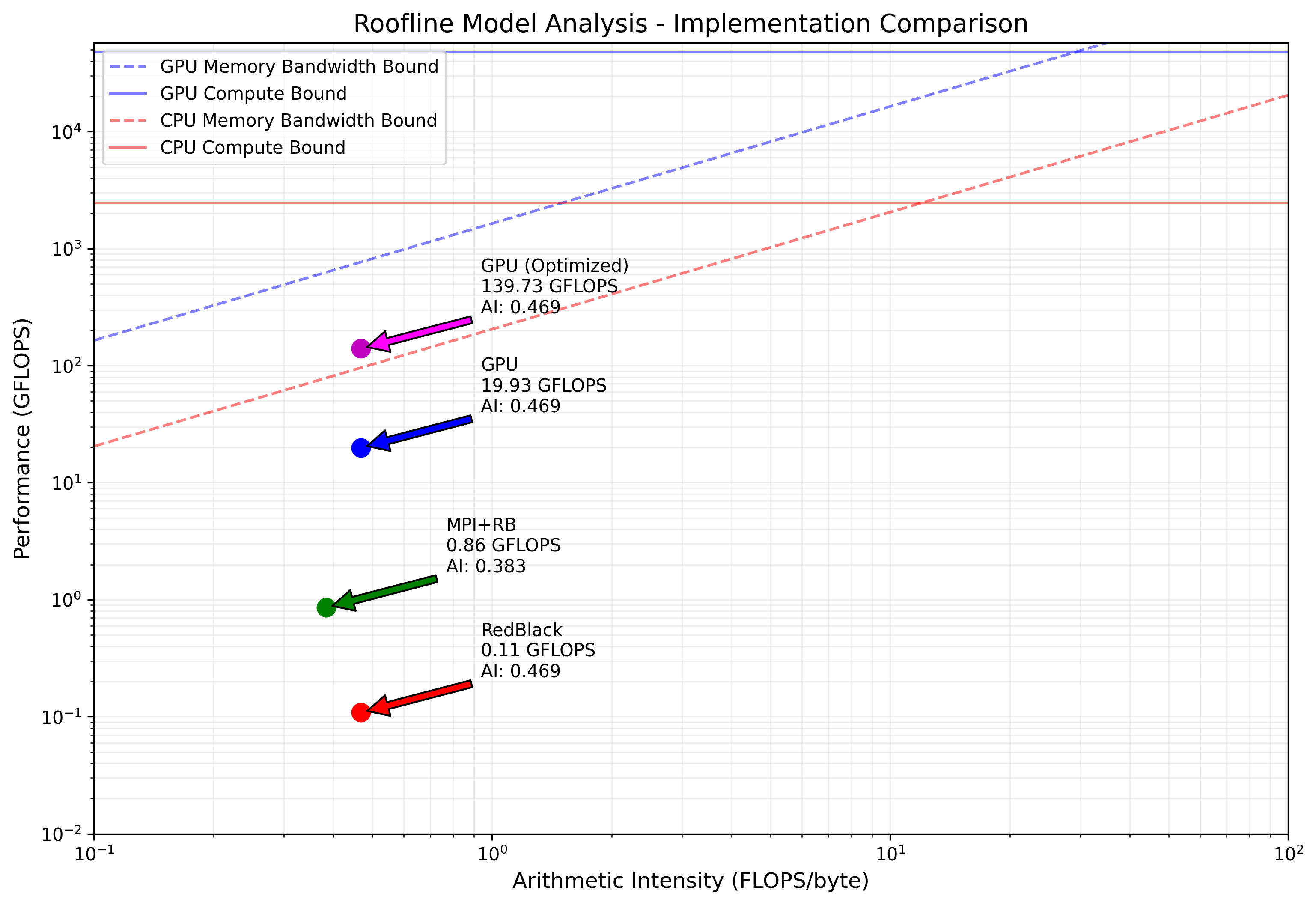
Roofline analysis reveals all implementations are memory-bound, operating below ridge points
My analysis reveals that all implementations are memory-bound, operating well below their respective ridge points (AMD MI250X GPU: 29.2 FLOPS/byte, AMD EPYC 7V13 CPU: 12.0 FLOPS/byte). This is expected given the nature of the Ising model computation, where each spin update requires reading multiple neighboring values but performs relatively few arithmetic operations.
The baseline GPU implementation achieves 19.93 GFLOPS with a memory bandwidth utilization of 42.52 GB/s. However, my optimized GPU implementation shows significant improvement, reaching 139.73 GFLOPS and 298.09 GB/s memory bandwidth, approximately a 7x performance increase.
The RedBlack CPU implementation operates at 0.11 GFLOPS with a memory bandwidth of 0.23 GB/s, while the MPI+RedBlack version achieves 0.86 GFLOPS and 2.24 GB/s memory bandwidth. Both CPU implementations show relatively low hardware utilization, suggesting potential for further optimization.
Scalability
Performance is evaluated across varying lattice sizes (64³ and 256³). Looking at my results, I see my optimized GPU implementation take 0.28s for a lattice size of 64³ and 5.5s for a lattice size of 256³.
While this is a 64x increase in lattice size, I only have a ~19.6x increase in runtime. This is a clear indication of my parallelization successfully scaling and improving at scale.
Implementation Comparison
My performance analysis reveals significant differences between implementations:
Serial vs. MPI: The single-rank MPI implementation performs similarly to the serial version (36.2s vs 35.6s), but scaling to 8 ranks yields a near-linear speedup, reducing runtime to 5.8s. This demonstrates effective parallelization with minimal overhead.
CPU vs. GPU: The baseline GPU implementation outperforms both serial and MPI versions significantly, completing the same workload in 0.95s. This represents a 38x speedup over serial and 6.1x over 8-rank MPI implementation.
Optimized GPU: My optimizations (shared memory, GPU-aware MPI, precomputed random numbers) further reduced the GPU runtime to 0.28s, achieving a 129x speedup over serial and a 3.4x improvement over the baseline GPU implementation.
Scaling Behavior: When increasing the problem size from 64³ to 256³ (64x more lattice points), the optimized GPU implementation shows excellent scaling, with runtime increasing only by a factor of 19.6 (from 0.28s to 5.5s).
The efficiency analysis shows that my optimized GPU implementation achieves the highest hardware utilization, though still well below theoretical peaks due to the memory-bound nature of the algorithm. The MPI implementation demonstrates good scaling but is limited by the AMD EPYC 7V13 CPU memory bandwidth, while the GPU implementations benefit from the significantly higher memory bandwidth available on the AMD MI250X GPU accelerator.
[7] results
Energy and Magnetization
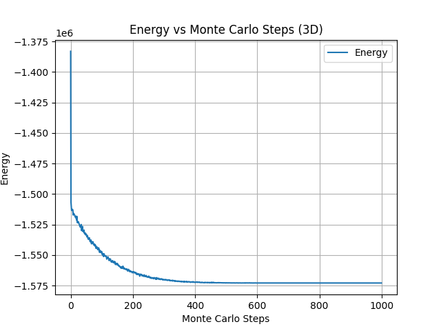
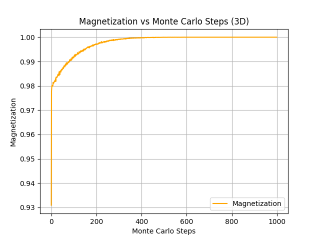
The energy and magnetization are plotted as functions of iteration count, demonstrating the convergence of the solution.
Energy vs iteration count showing system equilibrationMagnetization vs iteration count demonstrating convergence
Visualization
In addition to metadata, such as the energy and magnetization, I can also visualize the spins on the lattice.
The implementation and analysis of the 3D Ising model reveals several key insights about parallel computing strategies and their effectiveness. My results demonstrate that while both MPI and GPU implementations offer significant performance improvements over the serial version, the optimized GPU implementation provides the best performance, achieving a 129x speedup over the serial implementation.
Key Findings
Red-black update scheme successfully prevents pattern formation and enables parallel updates, proving essential for both MPI and GPU implementations
Memory access patterns significantly impact performance, as shown by the substantial improvements achieved through shared memory optimizations and GPU-aware MPI
Roofline analysis reveals that all implementations are memory-bound, suggesting that future optimizations should focus on improving memory access patterns rather than computational efficiency
Excellent scaling behavior of my optimized GPU implementation (19.6x increase in runtime for a 64x increase in problem size) indicates effective parallelization
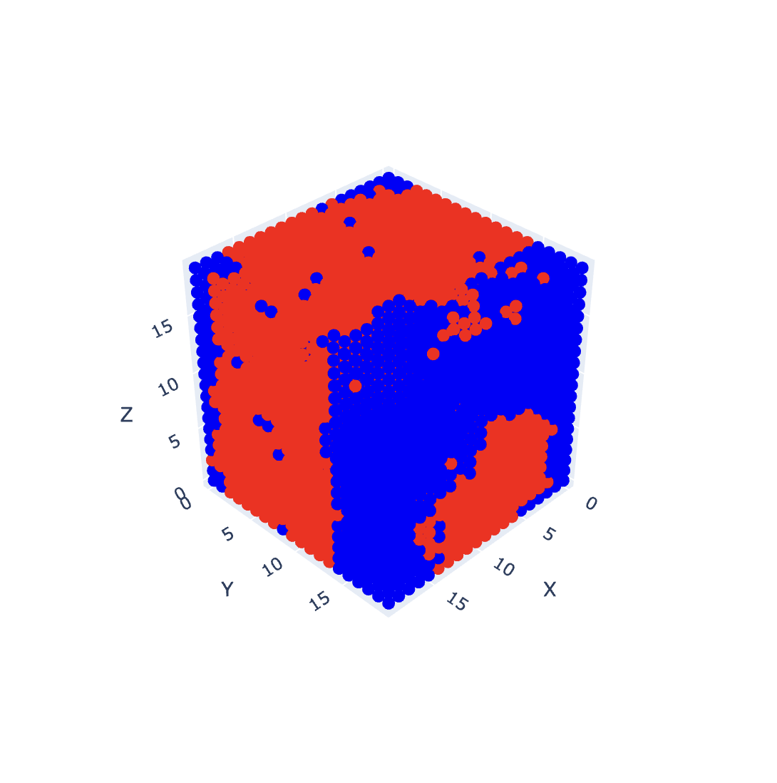
From a physics perspective, this simulation is being run at low temperature, and I am seeing spontaneous polarization! At high temperatures, I simply see thermal fluctuations. The visual demo is quite fun to play with.
[9] future directions
Pinned Memory
One promising avenue for optimization involves the implementation of pinned memory for GPU operations. Currently, my implementation uses pageable host memory for CPU-GPU transfers, which requires the CUDA driver to first copy the data to a temporary pinned buffer before transfer. By directly allocating pinned memory, I can eliminate this extra copy and achieve higher bandwidth for memory transfers.
Asynchronous Streams
A significant optimization opportunity lies in the implementation of asynchronous CUDA streams to overlap computation and communication. The current implementation processes halo exchanges and core computations sequentially, leading to idle GPU resources during communication phases. By dividing the computation domain into interior and boundary regions, I could compute the interior while simultaneously performing halo exchanges for the boundaries.
Temperature Scaling
From a physics perspective, extending the simulation to study temperature scaling effects would provide valuable insights into phase transitions. This would involve implementing an automated temperature sweep mechanism to observe the system's behavior around the critical temperature.
[10] conclusion
This project has successfully demonstrated the implementation and optimization of a 3D Ising Model using modern high-performance computing techniques. Through careful application of parallel computing strategies, I achieved significant performance improvements, with my optimized GPU implementation delivering a 129x speedup over the serial version. The combination of MPI domain decomposition and GPU acceleration proved particularly effective, allowing me to simulate larger systems with reasonable computational overhead.
My performance analysis revealed the critical role of memory access patterns in determining overall efficiency. The implementation of shared memory optimizations and GPU-aware MPI significantly reduced communication overhead, though the roofline analysis suggests potential for further improvements. The red-black update scheme proved essential for maintaining simulation accuracy while enabling parallel updates, demonstrating the importance of algorithm design in parallel implementations.
From a physics perspective, my implementation successfully captured the essential behavior of the 3D Ising model, including spontaneous magnetization at low temperatures and proper thermal fluctuations at higher temperatures. The interactive visualization tool provides an intuitive way to explore these phenomena, making the complex physics more accessible.
Looking forward, this work provides a foundation for future studies of more complex systems and optimization strategies. While I've achieved significant speedup, the identified optimization opportunities suggest exciting possibilities for even better performance in future implementations.
[11] appendix: gpu implementation details
GPU-Based Monte Carlo Implementation
GPU-Based Monte Carlo Implementation
1. Create 3D MPI Cartesian communicator
2. Assign GPUs to MPI ranks (round-robin)
3. Allocate GPU memory for spins, energy, magnetization
4. Initialize cuRAND states for each lattice site
For each Monte Carlo step:
    // Red-Black Update Pattern with GPU Acceleration
    For color in {red, black}:
        Launch GPU kernel with 3D thread blocks (8x8x8)
        For each site of current color (parallel):
            Calculate ΔE from 6 neighbors
            Generate random number using cuRAND
            If ΔE ≤ 0 or random < exp(-ΔE/k_BT):
                Flip spin atomically
        Copy spins CPU ↔ GPU
        Perform MPI halo exchange
        Copy updated halos CPU ↔ GPU
    // Energy Computation on GPU
    Launch reduction kernel with shared memory
    Compute local energy and magnetization
    MPI_Reduce for global observables
    If time to save:
        Gather lattice to rank 0
        Write configuration to file
GPU Energy Computation Kernel
GPU Energy Computation Kernel
1. Allocate shared memory for block-level reduction
For each thread in parallel:
    2. Calculate site energy from 6 neighbors
    3. Store in shared memory
4. Synchronize threads
For reduction stride = block_size/2 to 1:
    If thread_id < stride:
        5. Reduce energy values in shared memory
    6. Synchronize threads
If thread_id == 0:
    7. Atomic add block result to global counters
Special Thanks: Professor Grinberg for an excellent Parallel Computing on Heterogeneous (CPU+GPU) Systems course at Brown University!
Built for quantitative finance internship preparation, this card-based trading simulator implements real-time order matching, custom contract creation, and Monte Carlo AI strategies. Players trade futures contracts on card properties, with information revealing progressively through the game—combining expected value calculations with market microstructure analysis.
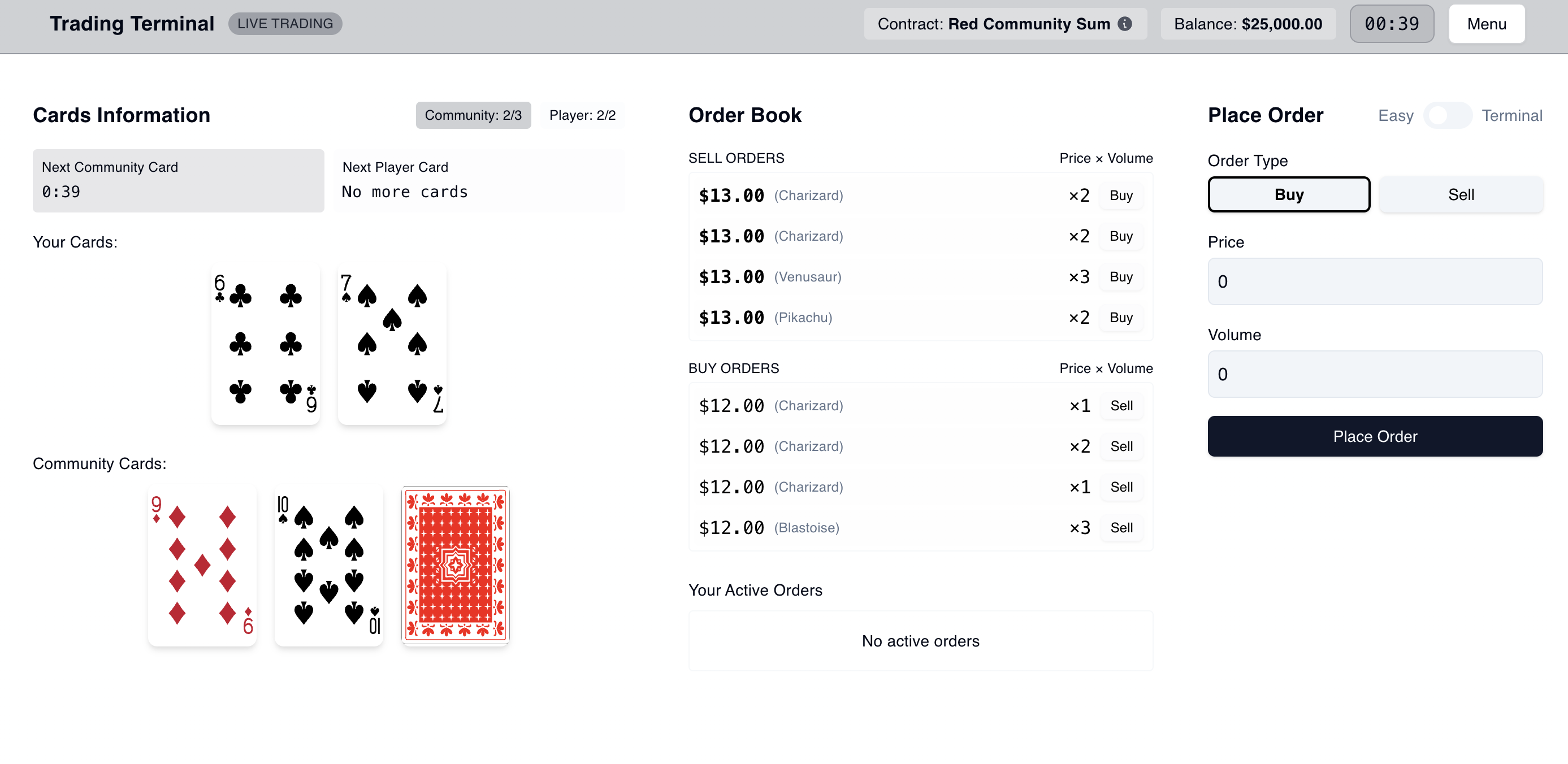
Live trading interface featuring real-time order book, market data, and trading controls
[2] system architecture
Electron Multi-Process Design
The application leverages Electron's architecture to separate concerns. The main process handles game state, AI execution, and order matching, while the renderer process manages UI and visualization. Secure IPC channels enable real-time market updates without blocking either process.
Game Phases
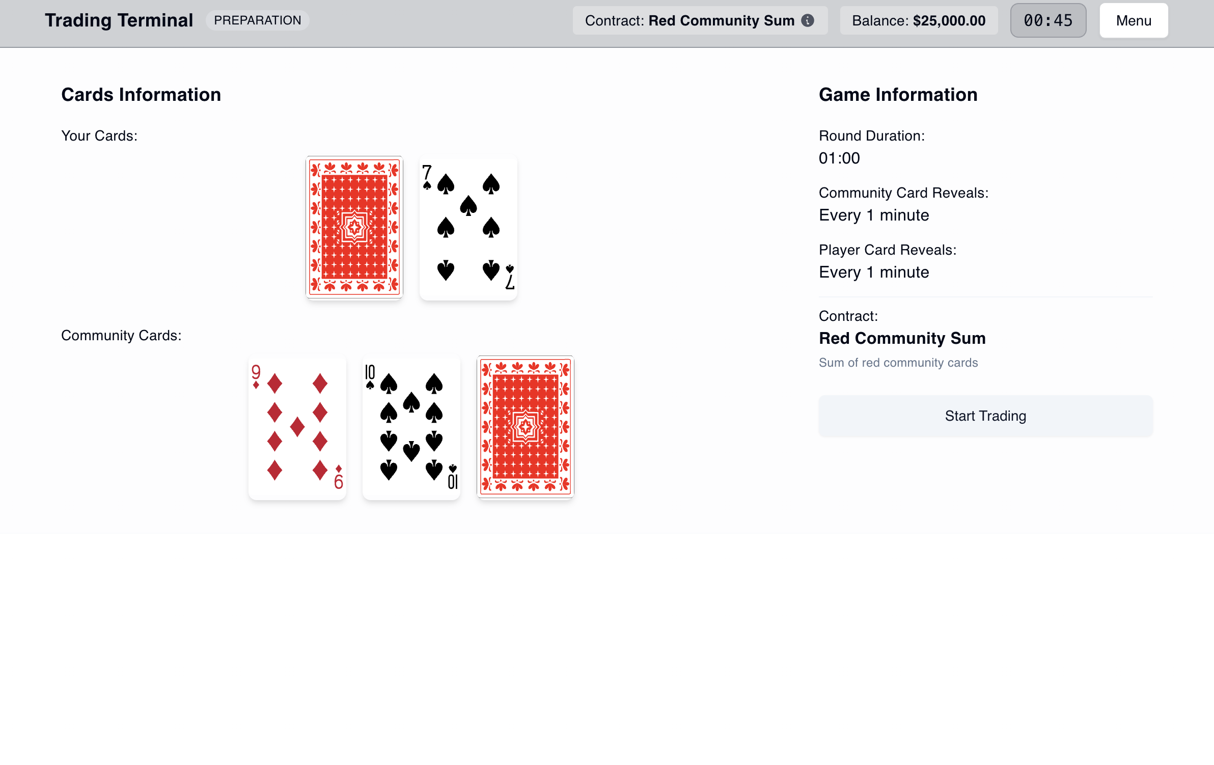
Preparation: Analyze initial card information before trading
The game progresses through four phases:
Configuration: Select active contracts and AI opponent strategies
Preparation: Analyze initial card information and contract values
Live Trading: Real-time order placement with continuous price discovery as cards reveal
Settlement: Calculate final contract values and P&L across all positions
[3] core implementation systems
Real-Time Order Matching Engine
The matching engine implements price-time priority: best prices execute first, then by arrival time at each level. The order book maintains separate buy/sell queues sorted by price and timestamp.
Order Matching Process
function matchOrder(newOrder):
    opposingOrders = getOpposingOrders(newOrder)
    sortedOrders = sortByPriceTimePriority(opposingOrders)

    for each existingOrder in sortedOrders:
        if newOrder.volume <= 0: break

        tradeVolume = min(newOrder.volume, existingOrder.volume)
        executeTrade(newOrder, existingOrder, tradeVolume)

        updateOrderStatus(existingOrder, tradeVolume)
        newOrder.volume -= tradeVolume

    broadcastMarketUpdate()
Large orders execute via partial fills across multiple counterparties at different price levels. The system supports market orders (immediate execution) and limit orders (rest in book until matched). IPC broadcasts market updates to all clients immediately, creating realistic bid-ask spreads through natural price-time priority dynamics.
Visual Contract Definition System
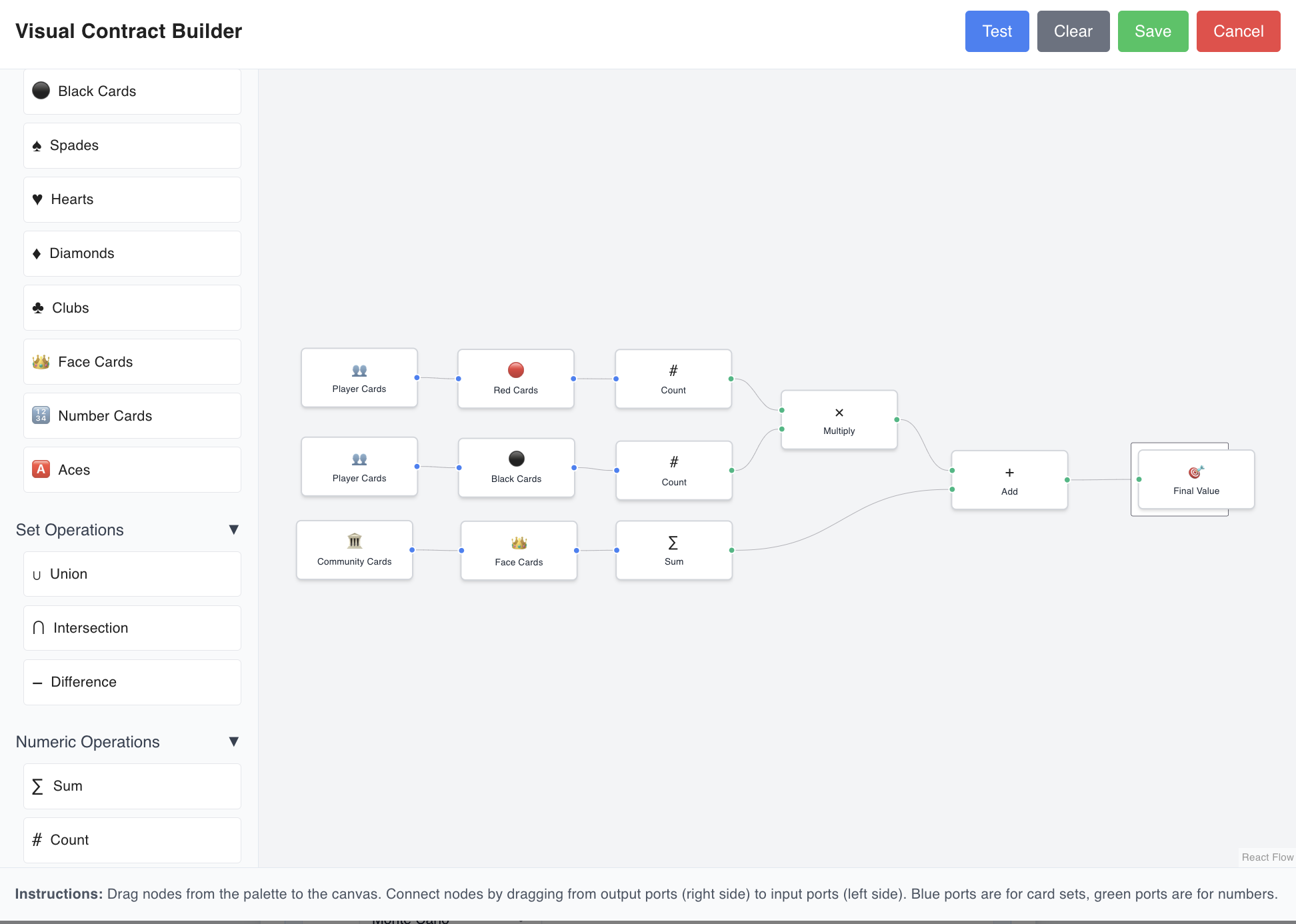
A node-based editor enables custom financial instruments via directed acyclic graphs. Players chain operations (data sources → filters → arithmetic → aggregations) to define contract payoffs without hard-coding.
Visual contract builder with drag-and-drop interface
Example Pipeline: "Sum of black community number cards"
Source: Community cards
Filter: Black cards
Filter: Number cards (exclude face)
Aggregate: Sum values
The evaluation engine performs topological sorting to determine execution order and validates dependencies before contract creation. Sequential evaluation maintains intermediate results, supporting branching logic for complex multi-operation contracts.
Monte Carlo AI Strategy
The AI uses pluggable strategies for market analysis. The Monte Carlo implementation estimates fair value through simulation, operating as an "anytime" algorithm where confidence improves with successive batches across trading turns.
The simulation identifies unknown cards not yet revealed, then generates thousands of scenarios by randomly distributing these unknowns. For each scenario, it calculates contract values and maintains a running average (fair value estimate) and variance (confidence measure). Higher confidence drives more aggressive trading behavior.
Monte Carlo simulation estimates contract values but misses a critical element: modeling adaptive opponents. The difficultly with creating a opponent model is that it is quite subjective and intuitive. It's a mix of logic and heuristics. Even with good microstructure, there is little to be gained playing against a opponent that cannot model your actions.
My proposed approach was quite Bayesian. For each agent, the goal is to build a probability distribution over the other agent's possible cards. Using this, when running a MC simulation, instead of using a uniform distribtion, we sample using the predicted probabilities, known as importance sampling. I think a Bayes net would be a solid architecture, with trades/initations as the observed variables. Even with this, there are a lot of varaibles to represent and the parameters might be hard to estimate.
However, this approach is quite computationally expensive and I did not have time to implement it. In the future, I would like to test this and see if it is sensible. Even still, I don't believe it will able to compete even close to a human trader, making it not very useful for practice.
Execution
The other issue was how to execute the orders. The Monte Carlo simulation provides a strong estimate of the fair value, but then the bot needs to execute the order. I implemented a few strategies for this, but this is bot dependent and does not have a single answer. On the bright side, this allows for diversity in the bots' behavior, and certainly has a lot of room for future improvement with interesting approaches.
[5] conclusion
Ultimately, while I don't believe this project helped improve my trading abilities, mainly due to the inability to model adaptive opponents, it was a valuable learning experience. I gained a good understanding of how markets function and how to build a trading system.
The goal of this project was to train a self-supervised learning model on the galaxy10_decals dataset, then use the learned encoder to train a downstream classifier. The dataset is a collection of 17,736 256×256 images of galaxies, with 10 different classes. I chose to use the MAE (Masked Autoencoder) architecture.
The encoder and decoder are both ViT models. I originally started implementing them from scratch, but later opted to use timm to load the models. This made them run much faster. For training, I created the actual task myself, but used stable-pretraining to help manage the training, do online probing, and implement early stopping.
I was limited on compute, so I was only able to test a few different configurations. Many hyperparameters were chosen from the paper, including the masking rate (0.75) and the learning rate/scheduler (cosine). Below are the results of the different configurations.
[2] what is a masked autoencoder (mae)?
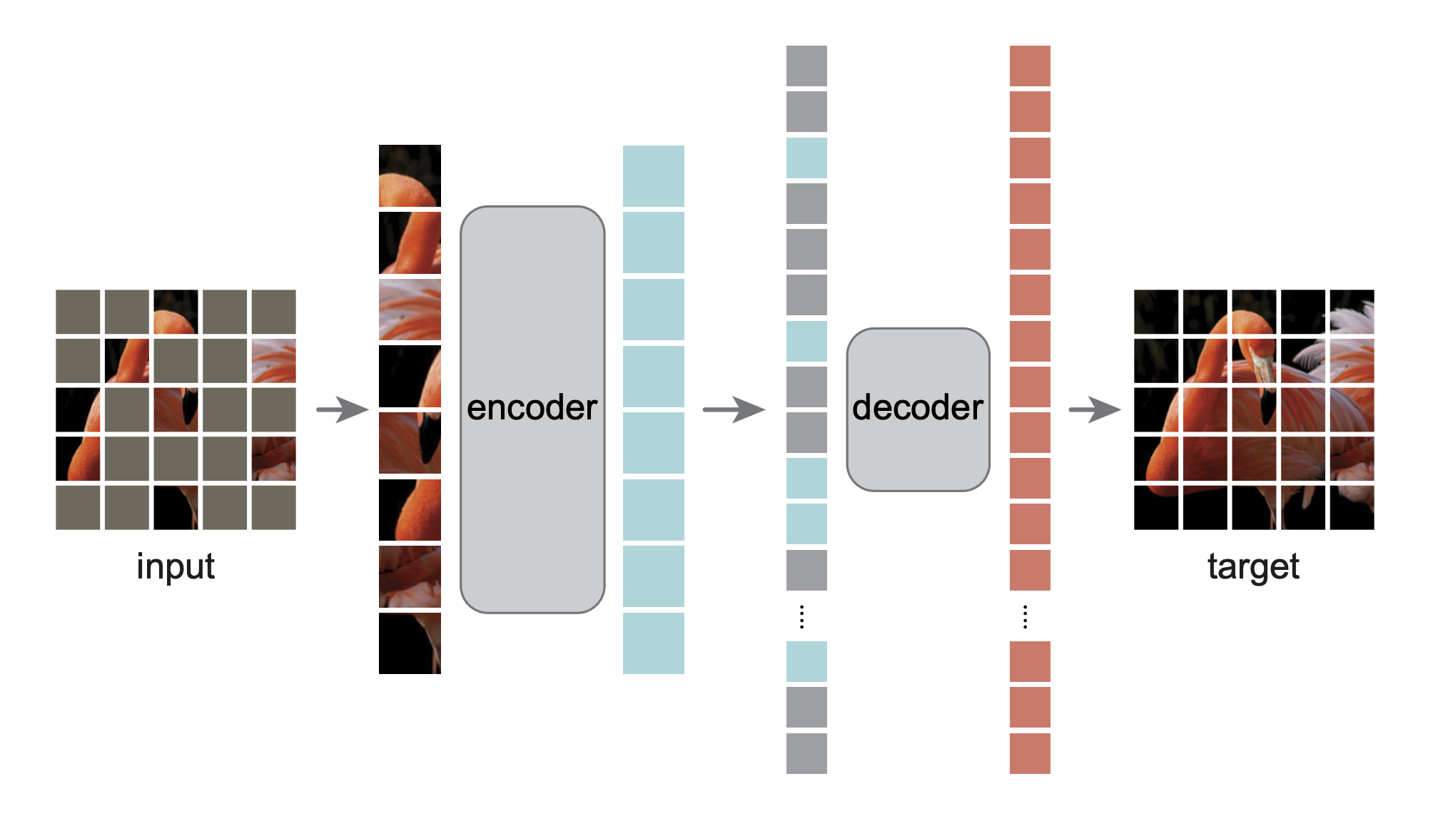
Masked Autoencoders are a self-supervised learning approach inspired by masked language modeling in NLP. The core idea: randomly mask out 75% of an image and train a model to reconstruct the missing pixels.
MAE architecture: an encoder processes only visible patches, while a lightweight decoder reconstructs the full image.
The architecture has two components:
Encoder (ViT): Processes only the 25% visible patches, learning rich representations from limited information
Decoder: Reconstructs all patches from the encoded visible patches plus learnable mask tokens
By solving this reconstruction task, the model learns meaningful representations of galaxy morphology (spirals, bars, bulges, mergers) without requiring labels. This learned representation can then be used for downstream classification tasks. Notably, for downstream tasks we really just care about building a strong encoder. In this training setup, because the encoder only processes the visible patches, we can train a much larger encoder than decoder, letting us create a more powerful model for cheaper.
[3] results
For comparison, I trained a supervised baseline, using the same architecture as the base model. I was able to achieve an accuracy of 68.25%, giving me a good comparison point.
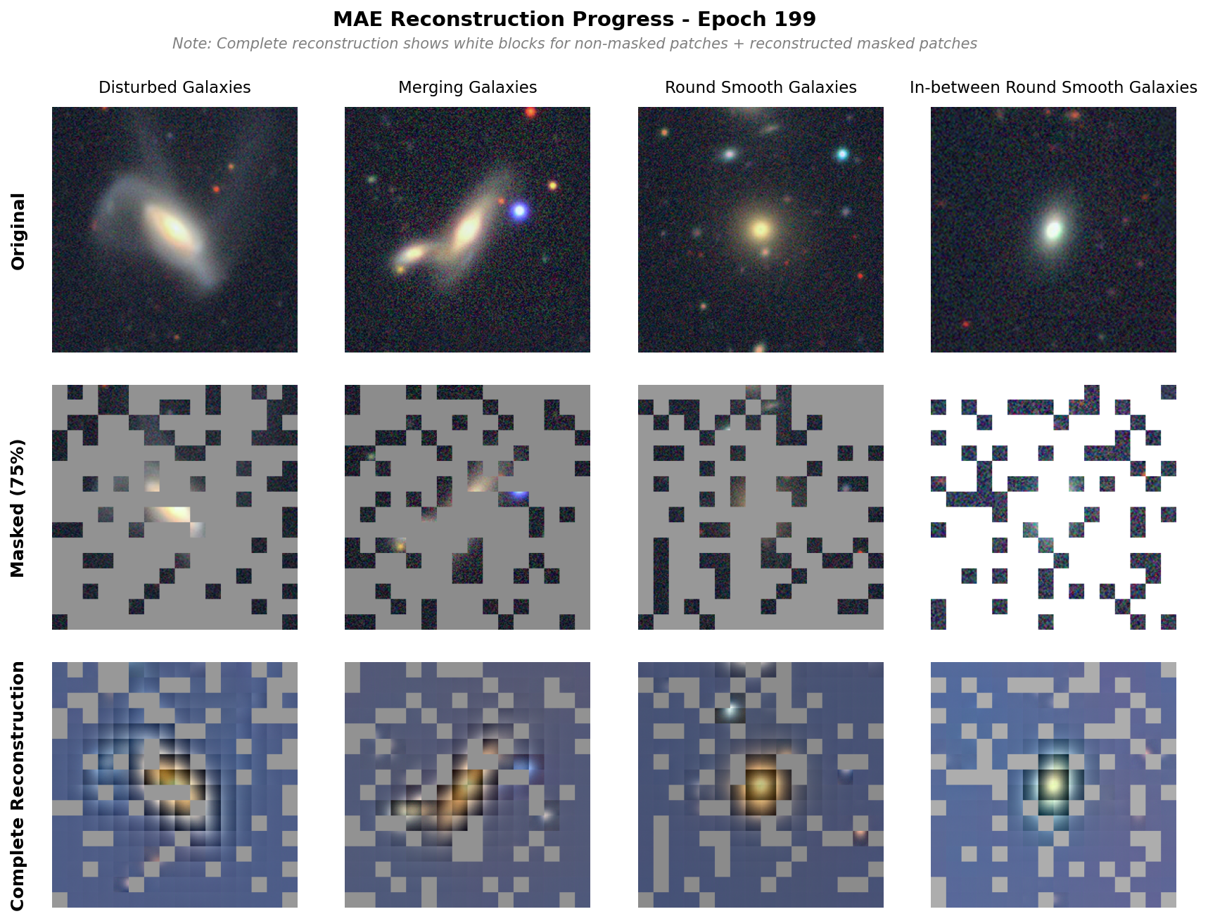
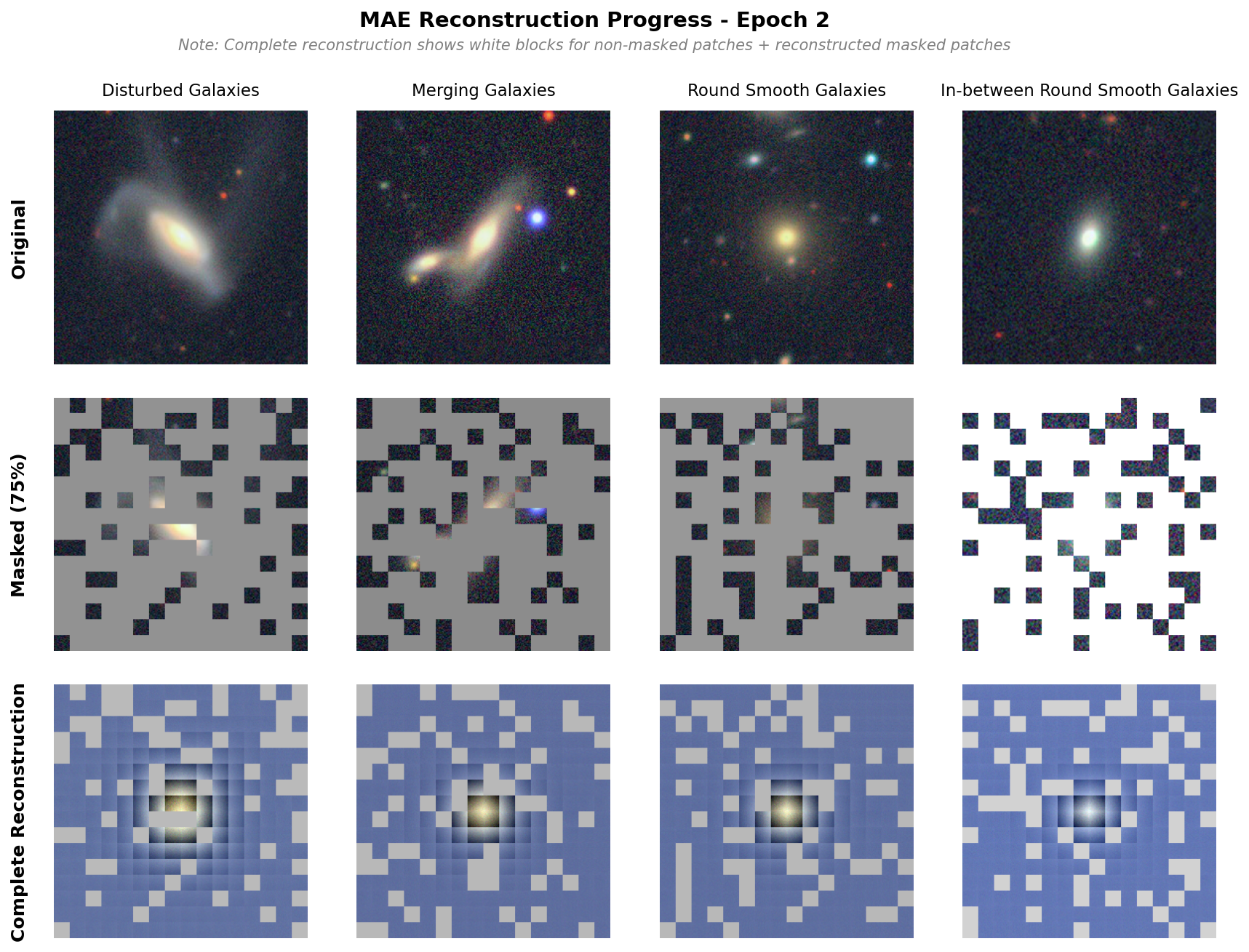
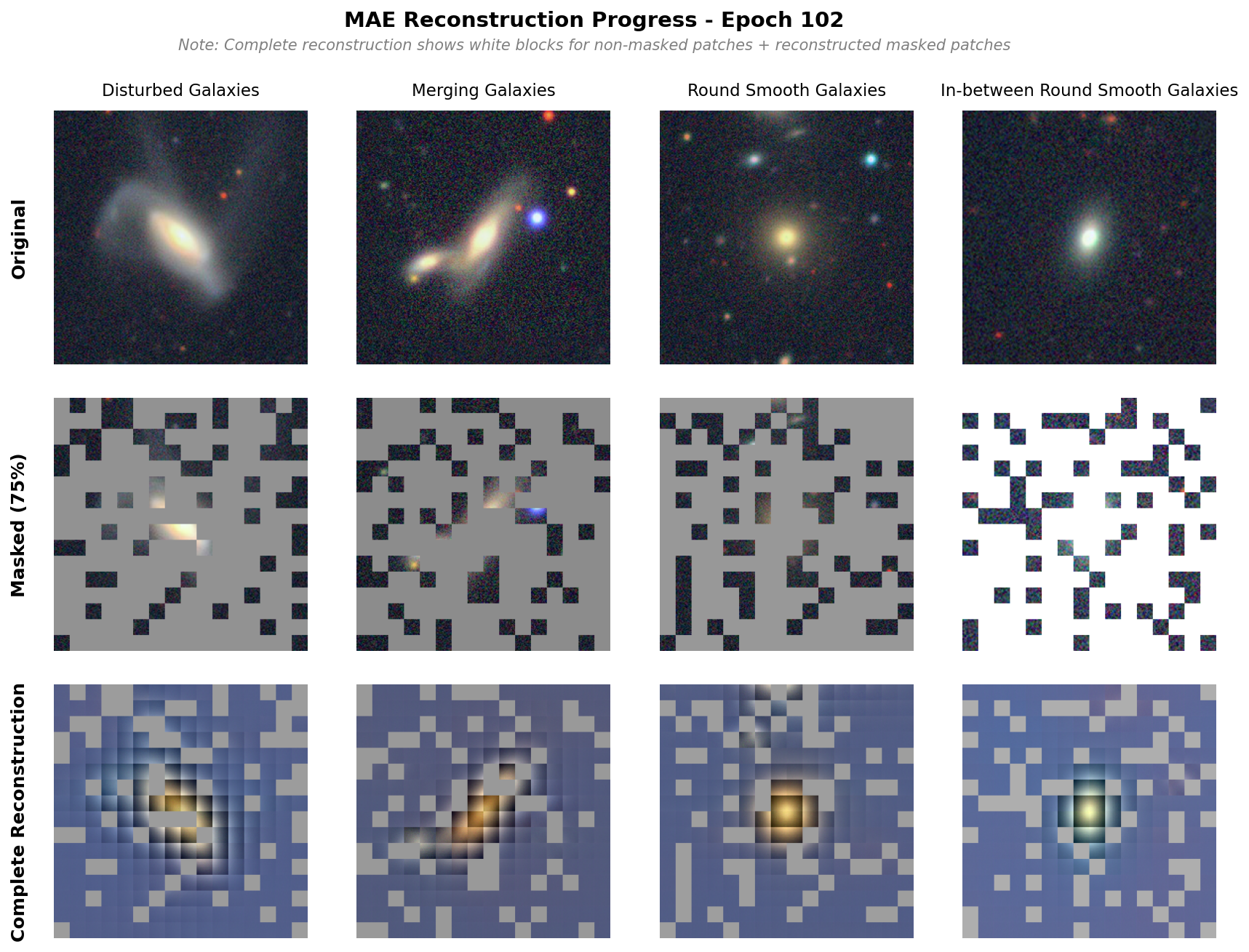
Below is an image of the reconstruction done by the base model. We observe pretty good reconstruction, though there are strong separations between each patch, which is less observed in the original paper. That said, we are able to see the galaxy shapes reconstructed well and subtle features (see the other galaxy in merging galaxy) also appearing.
Reconstruction
Model Size
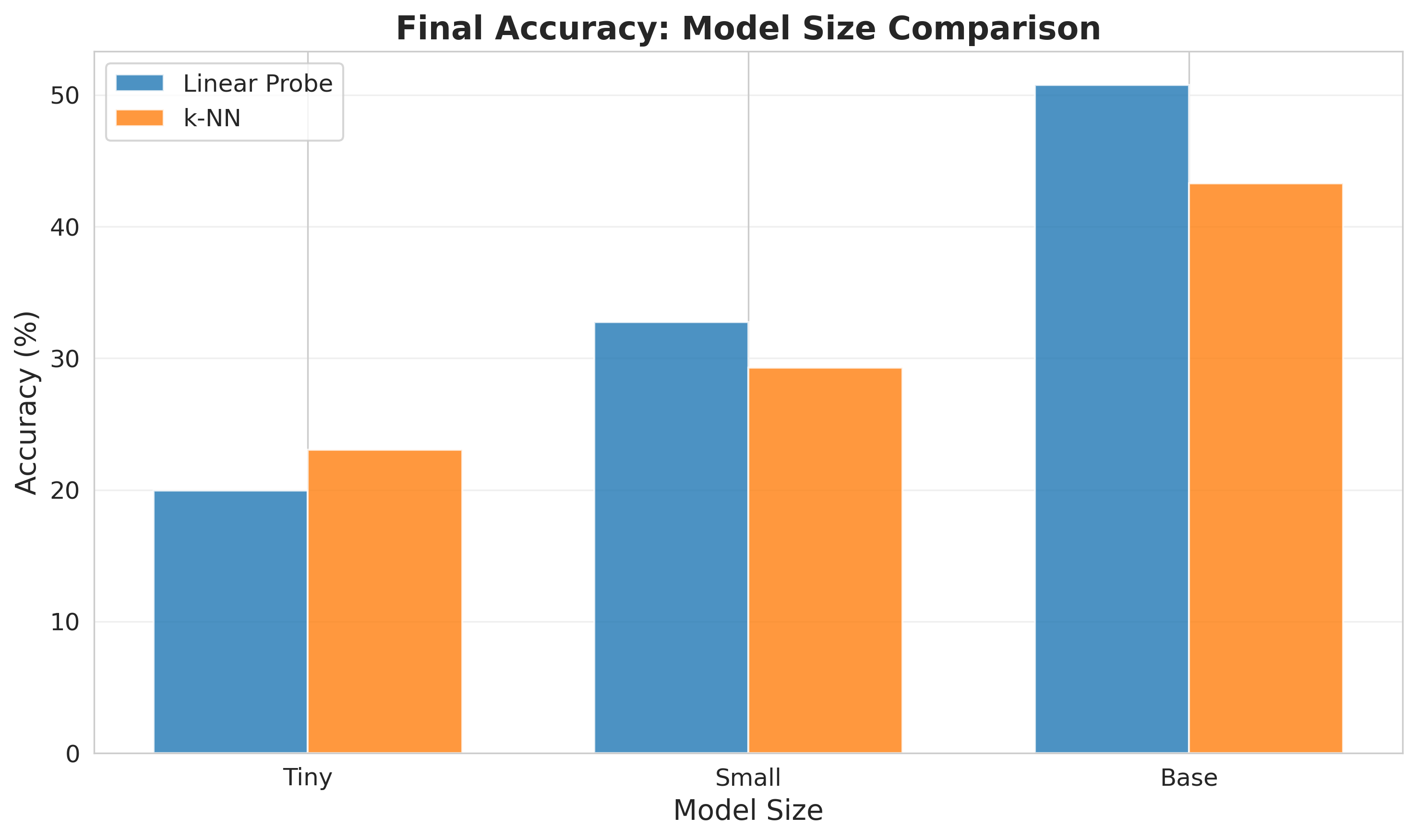
The first comparison I tried was changing the model size. This was also done to test our training pipeline quickly using small models, and is something I plan on doing in the future to give a good reference and confidence as we move to larger training runs. I tried three different sizes: a tiny architecture, a small architecture, and a base architecture. The results are shown below, showing both linear probe and k-NN results from the latent space. We see an increase in performance as the model size increases, and the trend suggests that even larger models would continue to improve performance. Our base model achieves an accuracy of 50.78%.
Model Size Results
Augmentations
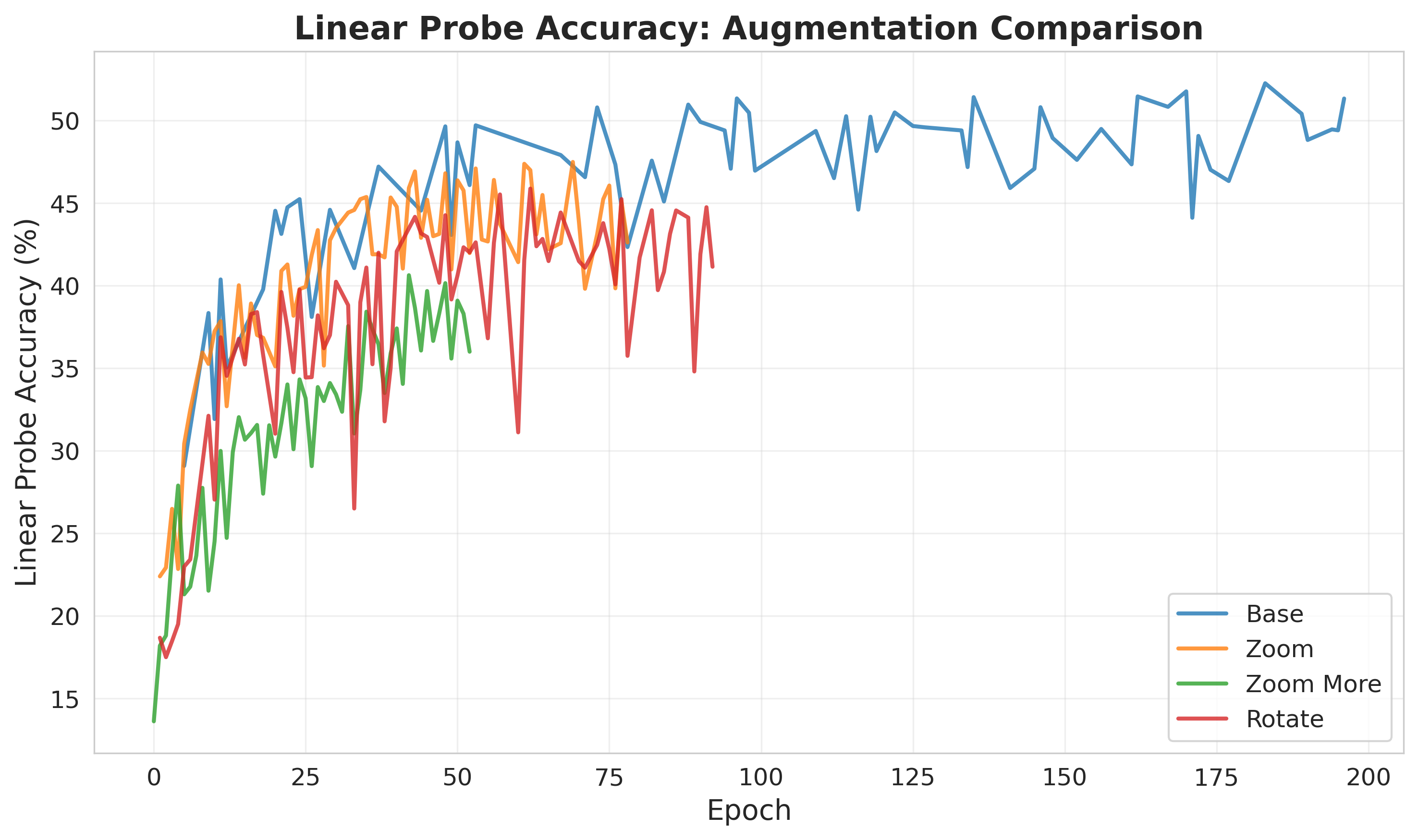
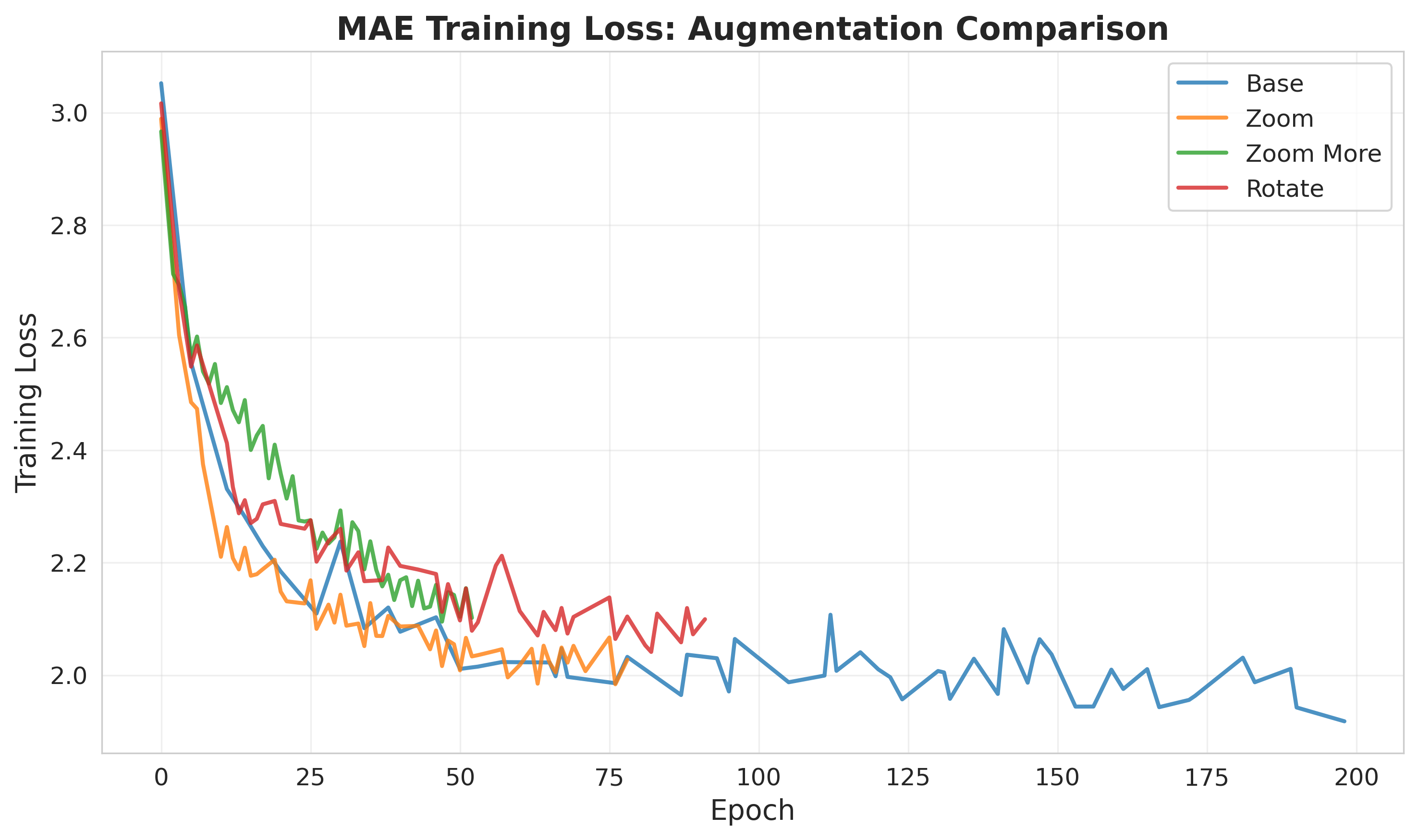
Next, I tried various augmentations. In the MAE paper, they note that the model performs very well without augmentations, but also does slightly better with augmentations. Noticing the galaxies were really just the center of the image, and there was lots of reconstruction wasted on predicting space (basically just noise). The augmentations are applied to the mae task, but the linear probes are trained on the original images. Below are the online linear probe results for the different augmentations. Notably, the augmentations do not improve the performance.
Augmentations Online Linear Probe Results
Downstream Architectures
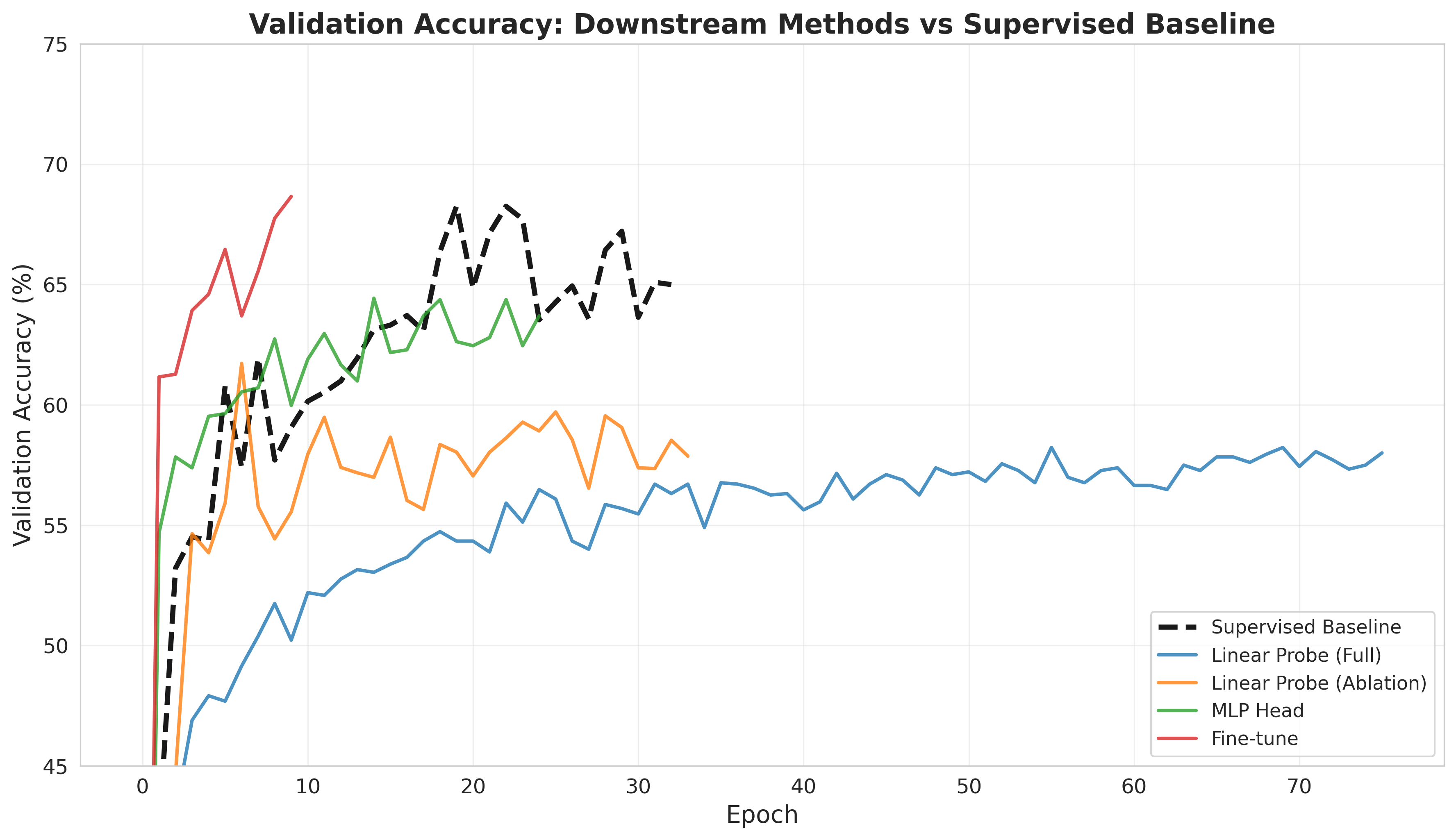
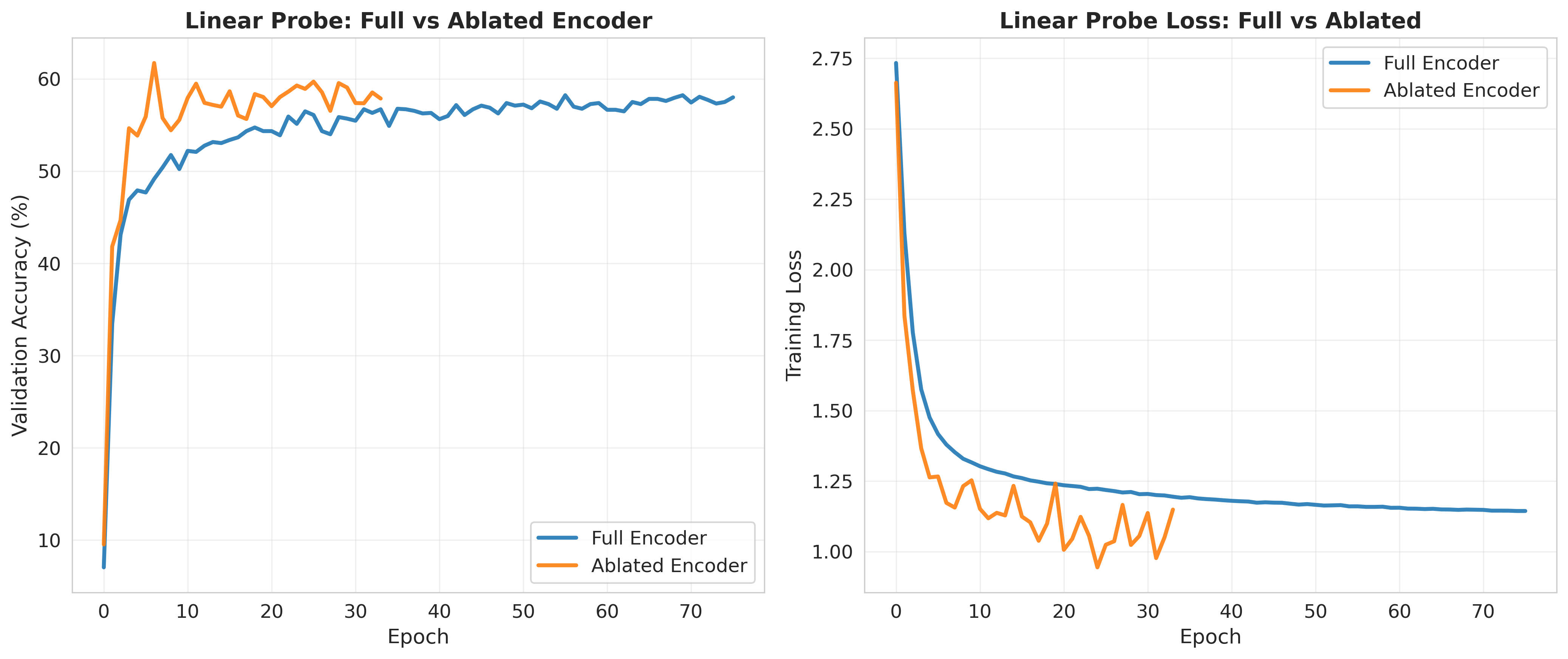
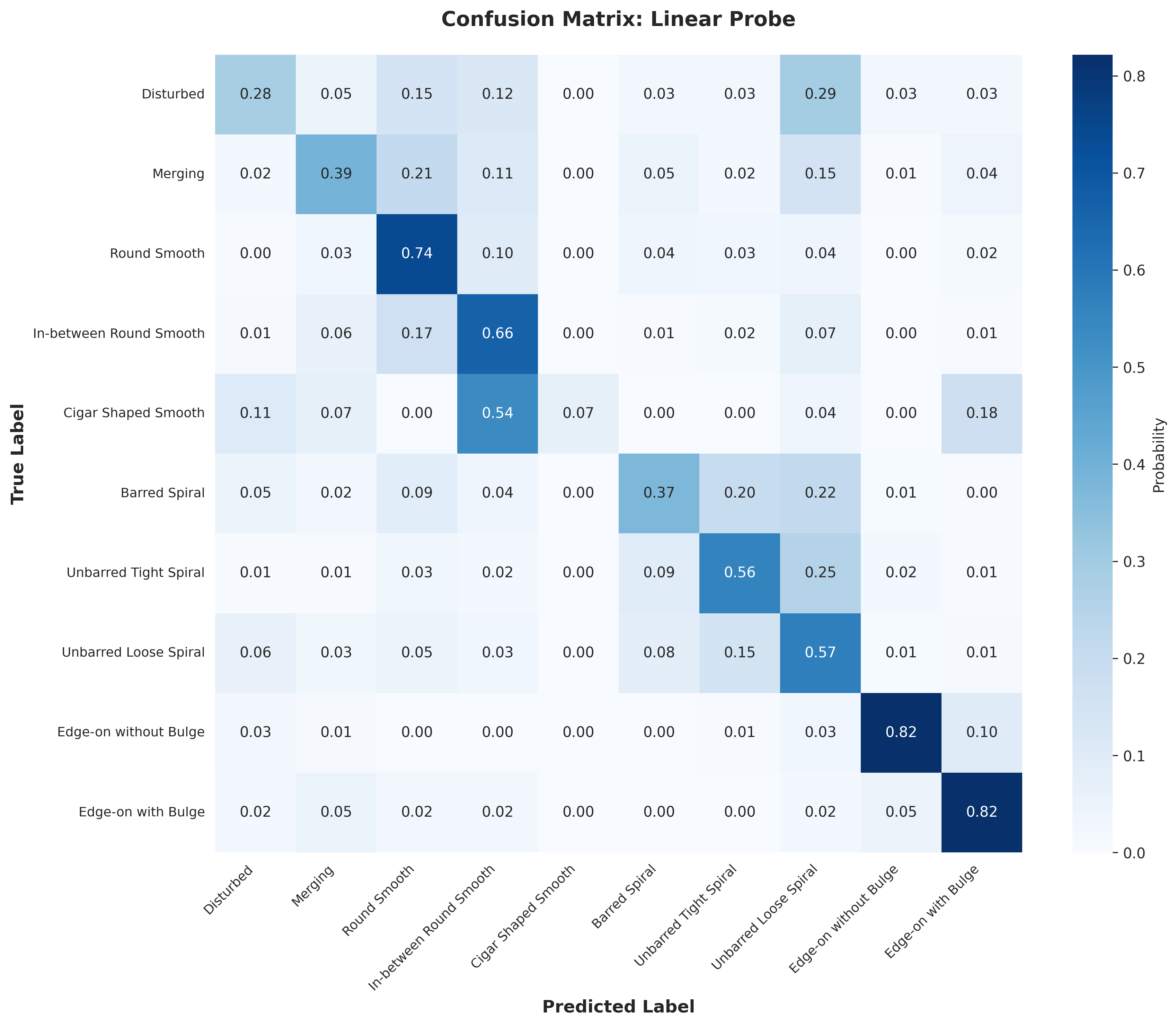
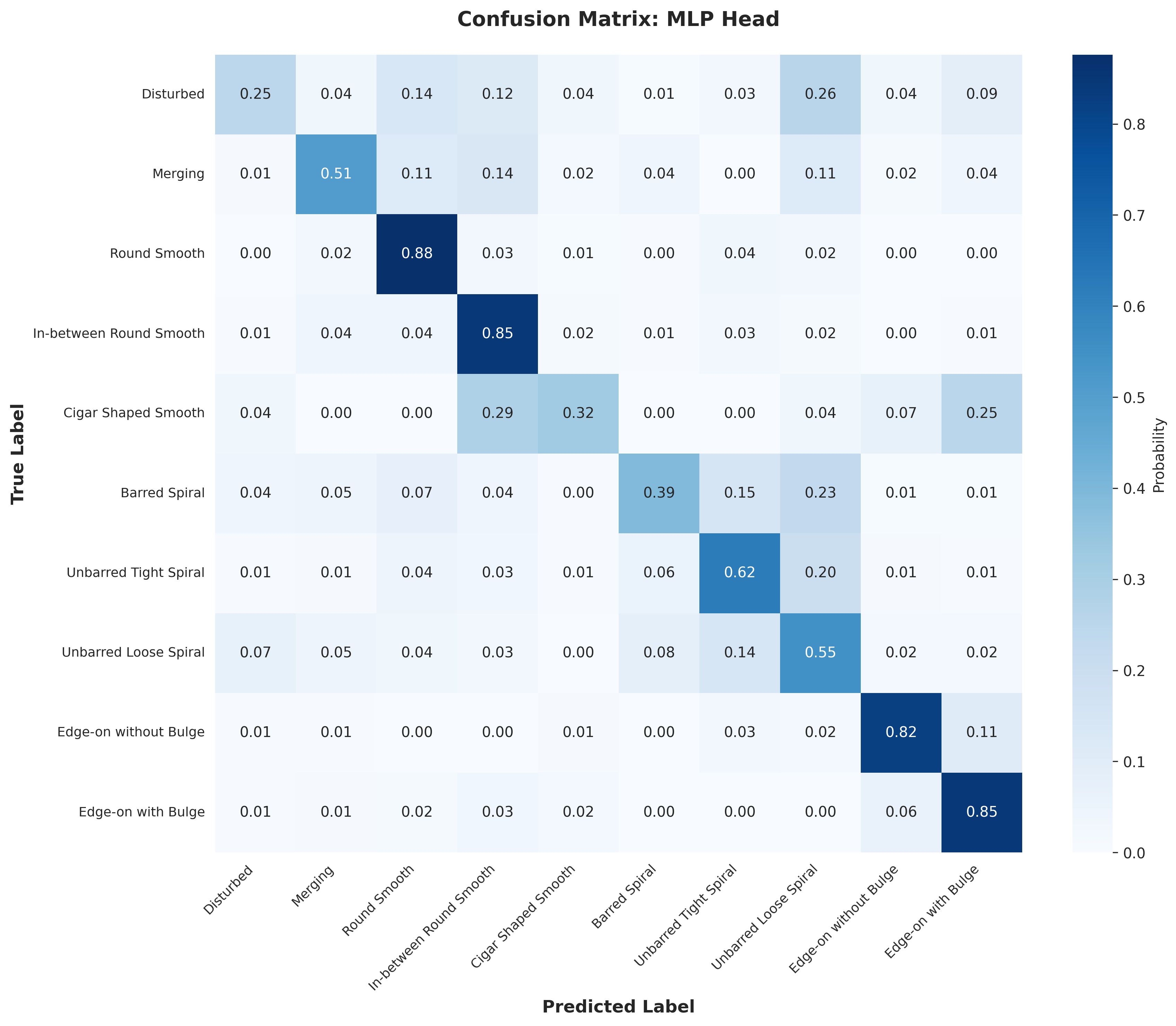
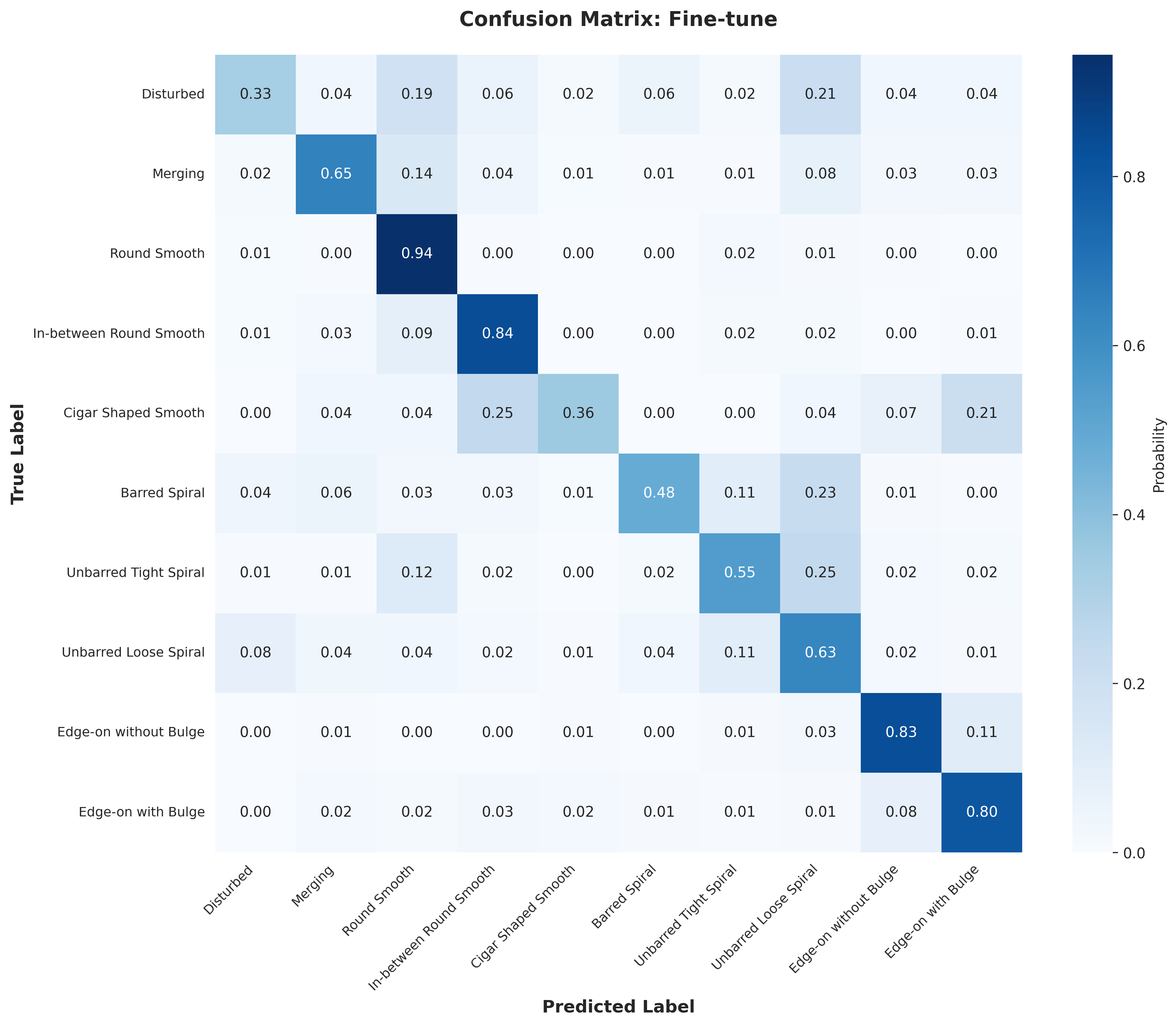
Lastly, using the base model, I tried various downstream architectures to take our latent representation from the encoder and train a classifier. I trained a linear probe on the final output and on the output ablated at depth 8 (out of 12) with the encoder frozen. I also trained a MLP on the final output with the frozen encoder and fine-tuned the model (with a mlp after the final output). Below are the results for the different downstream architectures. They start with the final epoch 199 base model. We see the fine-tuning reaches the same level as the supervised baseline in fewer epochs, the ablated linear probe does better than the nonablated linear probe, and the MLP does better than both linear probes. Overall, I was able to achieve an accuracy of 58% with a linear probe, 63.7% with an MLP, and 67.8% with fine-tuning. The fine-tuning was ended early, and likely would have reached the supervised baseline with more epochs.
Downstream Validation Accuracy
[4] discussion
Overall, the MAE was able to build a decent latent representation. I suspect with more compute we could get better performance. I would be interested in testing other parameters, especially the mask ratio. Nonetheless, our MAE was able to create representations comparable to the supervised baseline using small downstream models.
Weights and biases was a really useful tool for this project, and made it much easier to track and compare my different runs. stable-pretraining was also great for online probing and easy training. Visualizing the reconstruction was also helpful to get a holistic view of the model's performance (and just fun to look at). I also generated some confusion matrices (in the appendix) to get a better sense of the model's performance and found this to be insightful.
[5] figures
Reconstruction from Epoch 2Reconstruction from Epoch 102Augmentations Training LossLinear Probe Full vs AblationLinear Probe Confusion MatrixMLP Head Confusion MatrixFine-tune Confusion Matrix
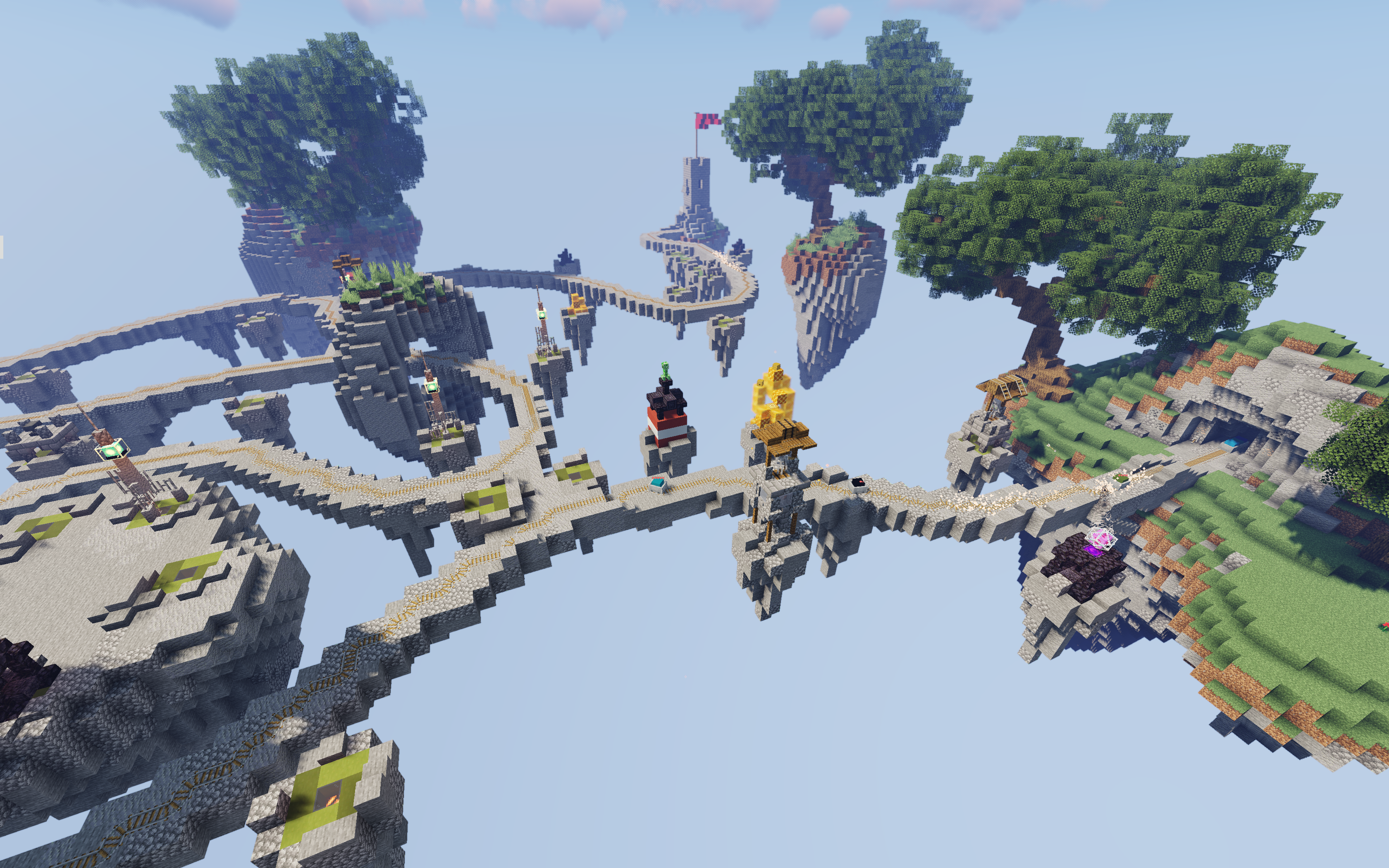
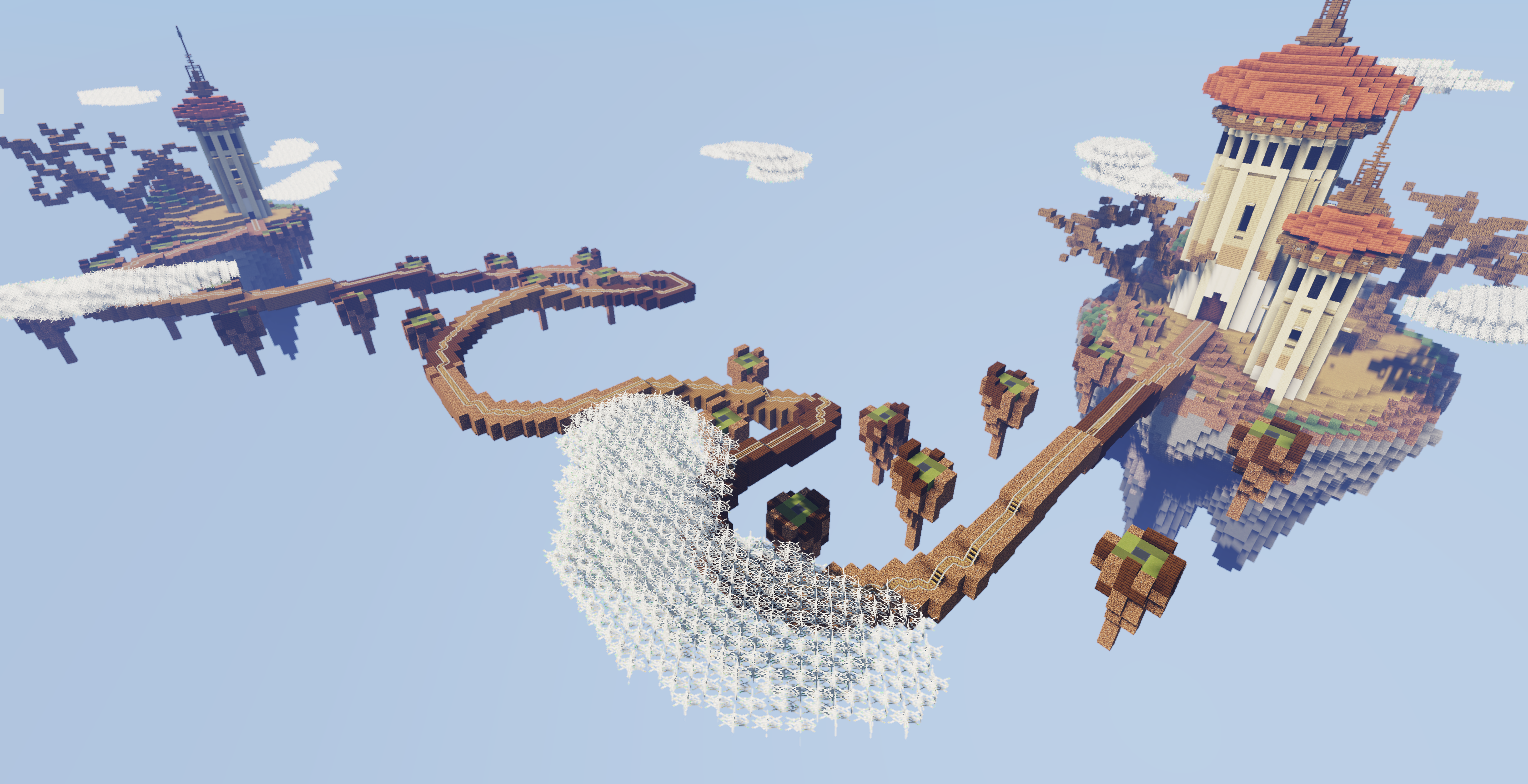
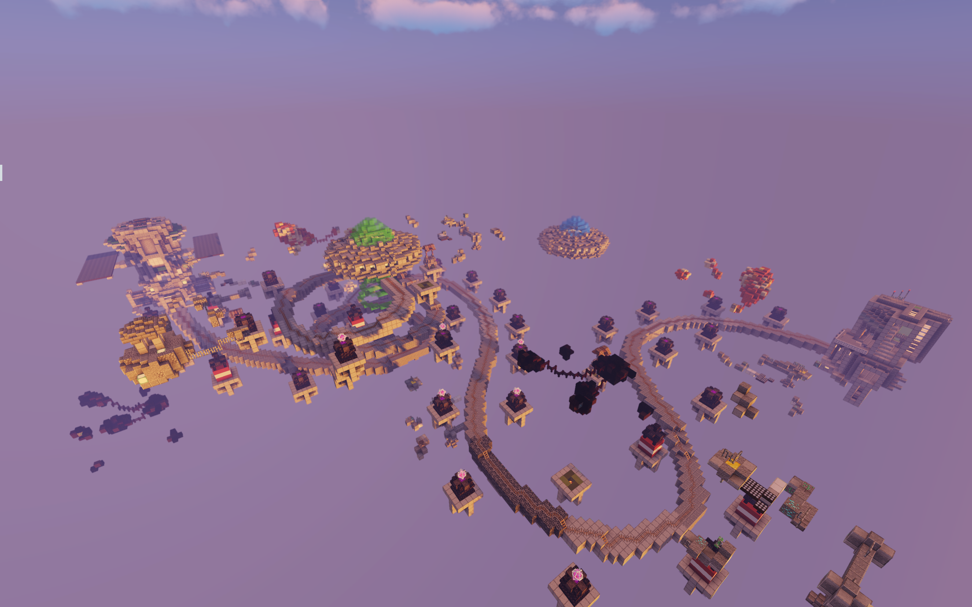
Games, physics simulations, and neural networks built entirely in Minecraft's native programming language, partnered with Microsoft
[1] introduction
I learned to code in Minecraft. Not with mods or plugins, but with mcfunction—the game's built-in command language. It's a bare-bones language with basic arithmetic (+, -, *, /, %), no variables (just "scoreboard" registers), and simple functions for interacting with the game world.
Nevertheless, these limitations provide a great foundation to build more complex things, as long as you get creative (get it). For example, there are no trigonometric functions, so to take the sine between two entities, you start at one entity, face the direction of the other, summon a new entity one block away, and the x/z coordinates are the sine and cosine.
To this day, this is still one of my all time favorite projects. At over 11,000 lines of code, this fully-featured tower defense game has players defend against waves of hostile minecarts using strategically placed towers. I drew inspiration the two tower defense games I loved the most growing up: Kingdom Rush and Bloons Tower Defense. It features six base tower types, each with three upgrade levels leading to two specialization branches with three unique abilities—creating 18 distinct tower variants. Players earn currency by eliminating minecarts and spend it to build or upgrade towers across multiple custom maps.
I wondered if Minecraft could simulate real physics. Of course, mcfunction has no calculus, no floating-point math, and no exponentials. However, even with calculus, some problems cannot be solved analytically. The solution is to use numerical methods. By discretizing time and replacing derivatives with finite differences, we can iteratively simulate differential equations.
The Newton-Raphson method captures this principle—iteratively improving approximations. For physics, we don't solve equations analytically; we step through time: Δx ≈ v · Δt.
Physics Implementation
The simulations implement gravitational attraction and aerodynamic drag using Euler integration:
For visualization, I use armor stands as particles. They store position data and automatically render in-game, providing built-in position tracking and smooth animation. Each tick, the simulation calculates forces, updates velocity and position, then applies the new position to the armor stand entity.
Challenges
Numerical precision: Minecraft scoreboards store only 32-bit integers. I scaled all values by 1000 (position 5.234 → 5234), giving three decimal places. Rounding errors accumulate, but careful timestep tuning helped with stability.
Collision singularities: When gravitating objects collide, r → 0 and force explodes. To solve this I dampen gravity disabled gravitational interactions at small scales. A collision system instead would be a fun future addition.
The system simulates both projectile motion with air resistance and n-body gravitational dynamics, where multiple objects create emergent orbital phenomena!
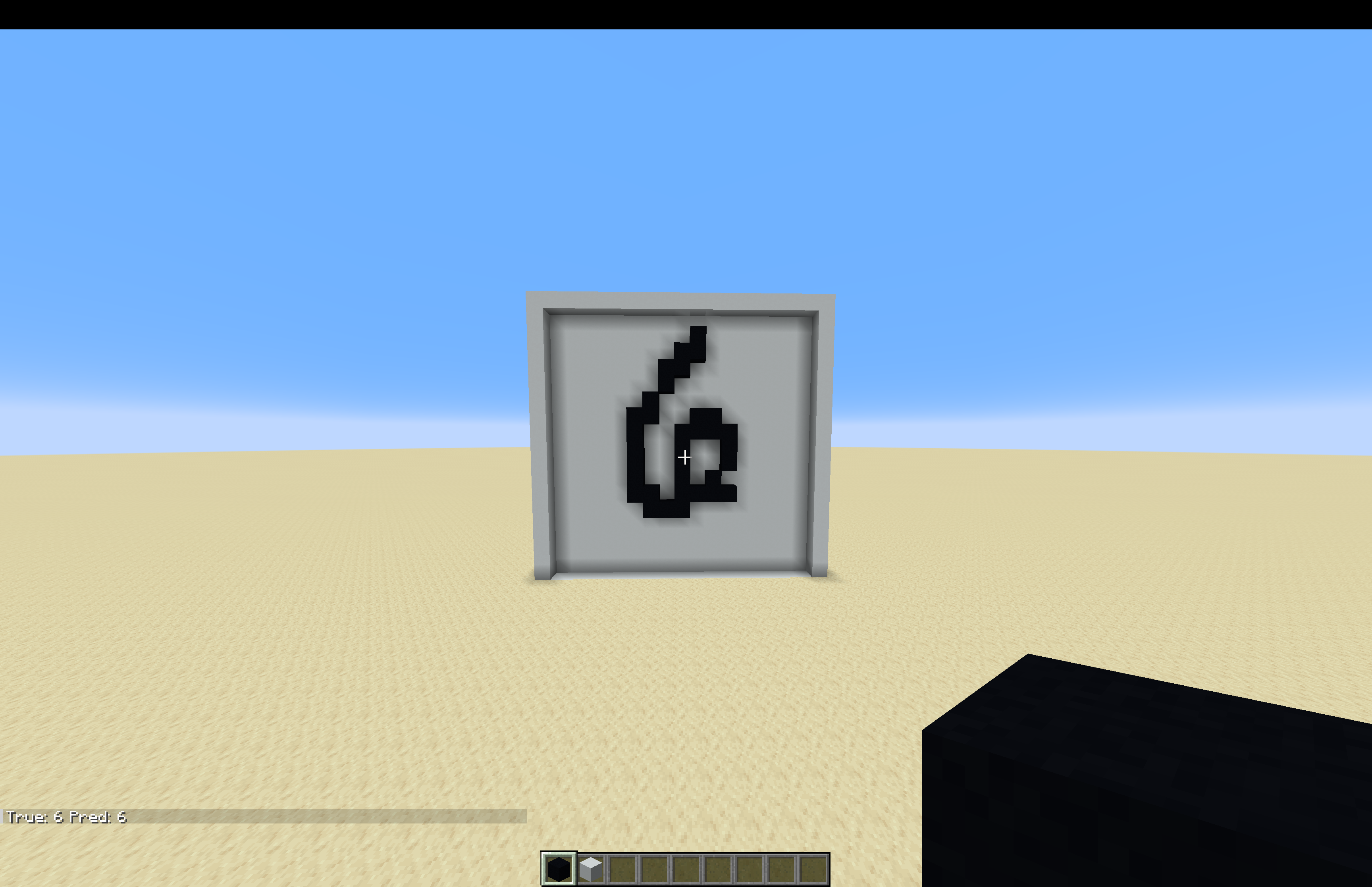
After taking a deep learning class, I wanted to implement a neural network in Minecraft. While the network is trained in Python, it is exported to mcfunction and runs inference entirely in vanilla Minecraft!
Live digit classification using a neural network running entirely in mcfunction
Pipeline
Training (Python): A simple MLP (784→32→16→10) trained on MNIST handwritten digits using TensorFlow. Preprocessing to binary values (fully white or black) ensures users can recreate digits with blocks.
Weight Extraction: Since mcfunction only has integers, I scale weights by 10,000 (0.7234 → 7234), preserving four decimal places. A Python script exports these scaled weights as scoreboard initialization commands.
Inference (Minecraft): Three operations implemented in mcfunction:
Matrix multiplication: Nested loops compute output[i] = Σ(input[j] × weight[i][j]) + bias[i] using multiply-accumulate operations. Fixed-point multiplication requires rescaling after each layer.
ReLU activation: Simple conditional: if neuron < 0, set to 0.
Softmax (approximated): Since we only need argmax and exponential is monotonic, skip the exponential entirely and just find the maximum output value.
Users draw digits on a 28×28 block grid, then run the predictor. The network reads the blocks, performs forward propagation through all layers, and displays the predicted digit. Despite crude integer arithmetic and approximated softmax, the system classifies accurately.
I am a huge fan of 3Blue1Brown's videos, and animated video essays in general, and I wanted to create a platform that would allow me to create similar videos for any topic. The landscape of education is rapidly evolving, moving toward more personalized and engaging learning experiences. As Sal Khan discusses in "Brave New Worlds," the future of education lies in creating content that adapts to individual learning styles and paces. All of 3Blue1Brown's videos are animated using a Python library called Manim. Since this is all text based, this is a great problem for language models!
So for Hack@Brown, I built Illuminate with a team. By combining the power of large language models with mathematical animation engines, we can automatically generate educational videos that explain any topic in an engaging, visual way!
[2] how it works
The AI Pipeline
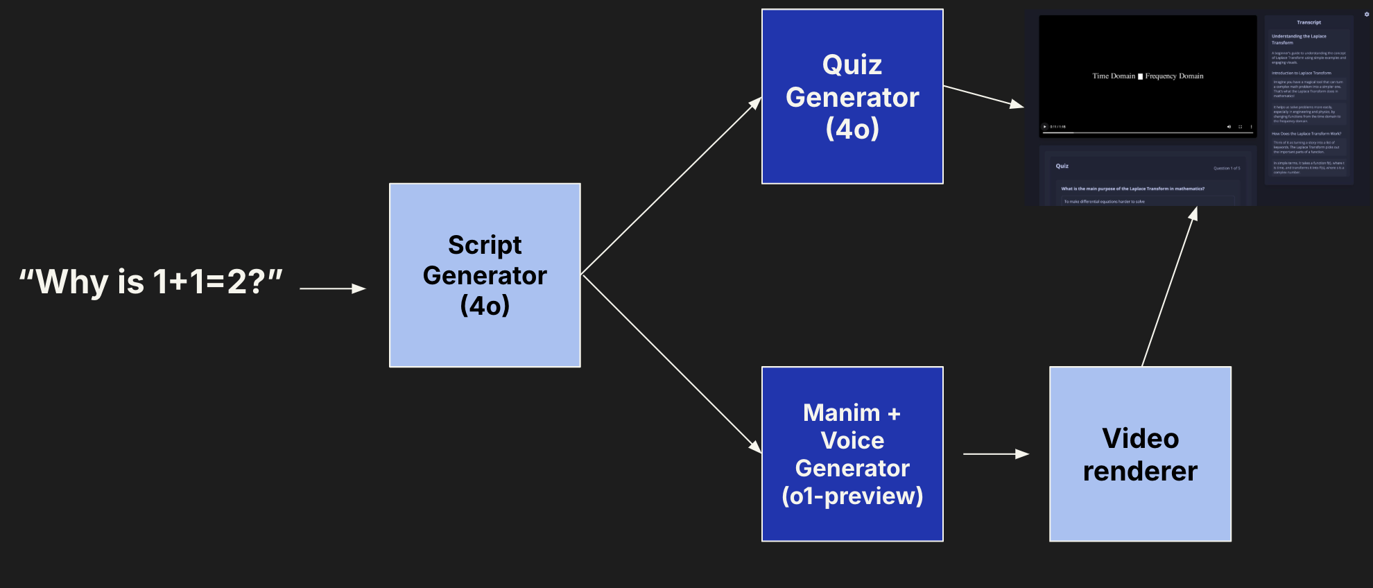
Illuminate uses a pipeline built with LangChain to orchestrate multiple AI services and steps. The process begins when a user inputs any topic they want to learn about. This simple prompt then flows through several stages that work together to create a complete educational experience.
The complete pipeline from user input to generated video and quiz
First, the input is processed by a script generator that creates a structured lesson plan, then iteratively refines it into a narrative script with suggested animation types and details. This script generation phase ensures that the content is pedagogically sound and follows a logical progression that builds understanding step by step.
Once the script is complete, a Manim generator takes over to create Python code for mathematical animations that will illustrate the concepts visually. This animation code generation process translates the abstract script descriptions into concrete visual representations. The code is then executed in a controlled environment to render the final animated video with synchronized voiceover. This is notably not a DAG. If the generation is successful, the video is shown to the user. Otherwise, the model takes the error and iterates on the code.
Simultaneously, a separate AI process generates interactive quiz questions, multiple choice options, and detailed solutions to test the user's understanding of the material.
Technical Architecture
Backend Infrastructure: The backend is built using modern AI and web technologies. LangChain orchestrates the entire AI pipeline and FastAPI provides a backend API framework that handles requests and responses efficiently. The system leverages OpenAI GPT models to power both content generation and script creation.
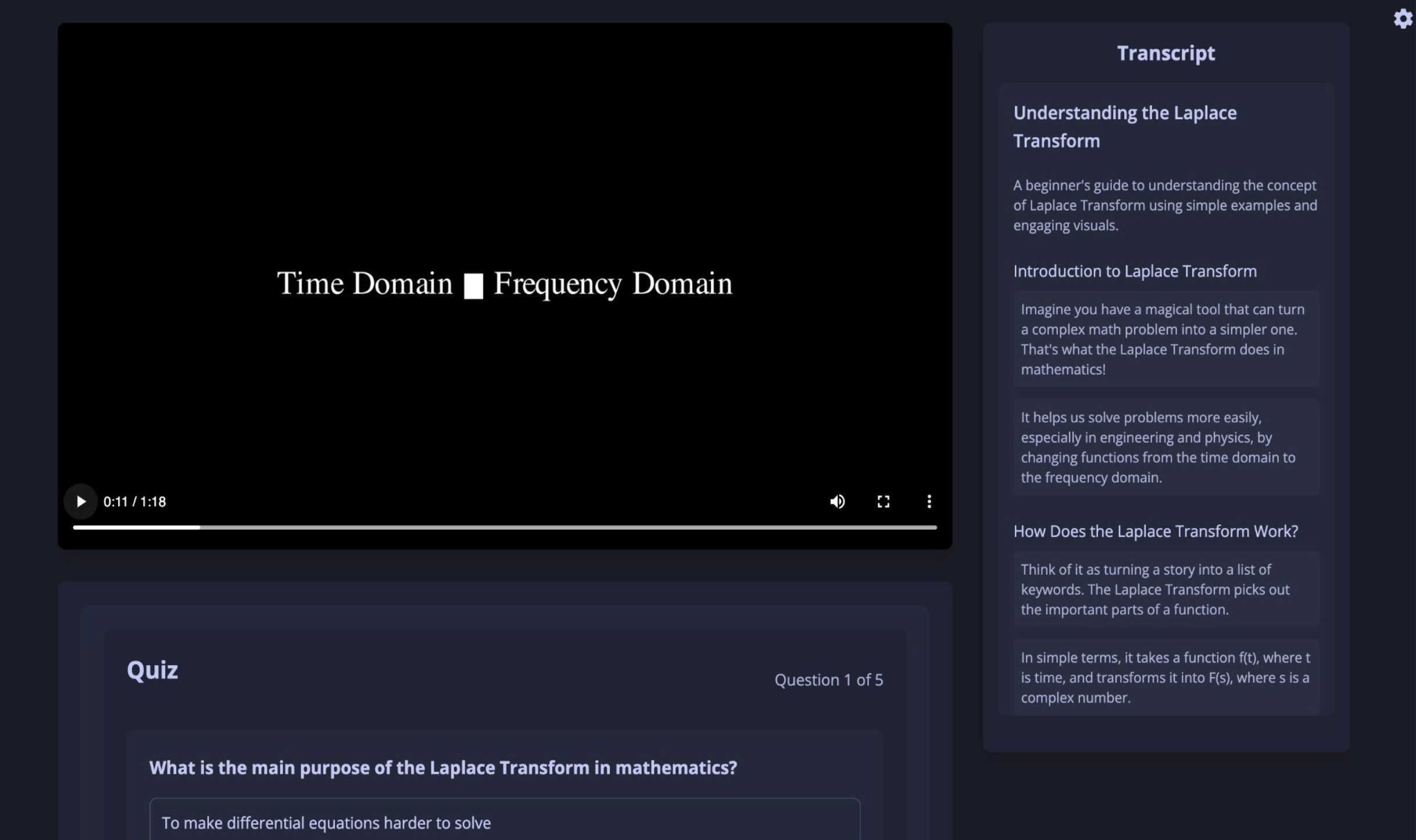
Frontend Experience: The user interface is built with React. Real-time integration ensures seamless communication between the frontend and backend services. Once generated, the platform shows the video, a script on the side for accessibility, and a quiz below.
Animation Engine: At the heart of the visual experience is Manim, the Mathematical Animation Engine that creates high-quality educational animations capable of illustrating complex concepts through motion and visual storytelling. The system allows for customizable animations and a voiceover generator. The built in voiceover allows synchronous narration with the animations.
The main interface
[3] technical challenges
AI Code Generation
One of the most significant challenges was getting large language models to generate reliable Manim animation code. The models often struggled with creating syntactically correct Python code that would execute without errors, particularly when dealing with the specific syntax requirements and object-oriented structure that Manim demands. Additionally, ensuring that animations didn't overlap or conflict with each other required careful prompt engineering and validation logic. Maintaining proper timing and synchronization between visual elements and the narrative flow proved especially difficult, as the AI needed to understand not just what to animate, but when and for how long each element should appear. Finally, including all necessary voiceover elements and ensuring they aligned perfectly with the visual timeline required multiple iterations and refinement of the generation process. This is still a work in progress and will require more research and testing for stable and robust results.
Manim Code Execution
Manim requires a few libraries that are tricky to run in different environments. Knowing this would have saved a lot of time and frustration. Eventually, we migrated to using a Docker container to run Manim, which made it much easier to run.
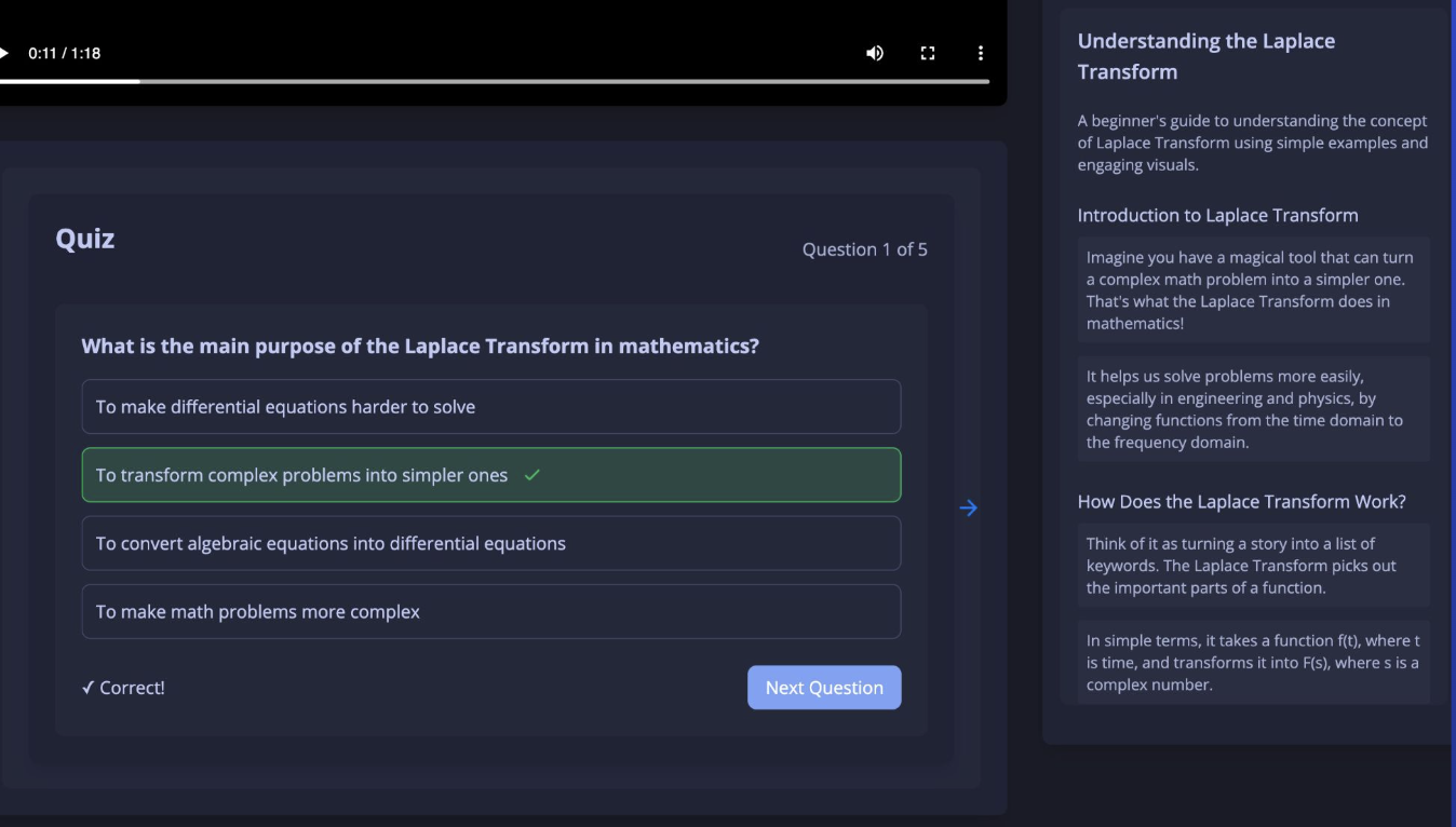
Interactive quizzes test understanding and reinforce learning
[4] impact and future directions
Educational Potential
Illuminate represents a step toward making high-quality educational content more accessible. By automating the creation of animated explanations, we can help educators and learners focus on understanding rather than content creation.
Future Enhancements
We won best use of GenAI at Hack@Brown, but there are a lot of future steps required to make this a truly useful tool. While fun to experiment with, the generation quality is still poor. That said, I still believe the concept is valuable and has potential. With this in mind, here are some future steps:
Use a VLM to inspect generated videos and imrove them iteratively before returning to the user.
Allow follow-up questions during video playback.
Accept images, diagrams, or documents as input to generate more contextual educational content.
Learn from user interactions and quiz performance to improve future content generation
Allow for multiple languages. This should be realtively easy with some translation tools.
An LLM-powered teaching assistant that adapts to course material to guide students through conceptual and technical questions
[1] the challenge in modern education
As both students and teaching assistants in the Brown CS department, we experienced firsthand the issues facing modern education. Students struggle to receive the help they need to learn effectively, complaining about long wait times, while TAs are overwhelmed with too many students.
Before coding this project, I created a survey to get an understanding of students' use of AI and views on current office hours. While expected, our research was still surprising: 79% of students report using ChatGPT before going to office hours, and 50% use it before even trying EdStem (Brown's Q&A system). Meanwhile, two-thirds of TAs report being asked the same questions repeatedly, creating an inefficient cycle that leaves everyone frustrated.
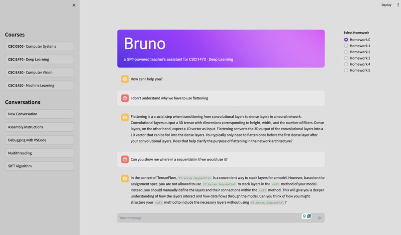
The ATA interface provides course-specific help and guidance
Students reported facing long waits, feeling pressured to ask questions quickly, and often receiving incomplete answers. When they can't get help, they turn to generic AI tools that don't understand their specific course context or pedagogical goals. This creates a gap between what students need and what they can access.
[2] a course-specific solution
The ATA Approach
Unlike generic AI tools, ATA (Artificial Teaching Assistant) is designed specifically for educational environments. It uses retrieval augmented generation (RAG) to access relevant course materials including syllabi, assignment specifications, code examples, and even previous EdStem discussions.
The key innovation is course adaptation - ATA doesn't just answer questions, it provides responses informed by the specific context of each course, ensuring students get help that aligns with their instructor's teaching goals and assignment requirements.
Pedagogical Design
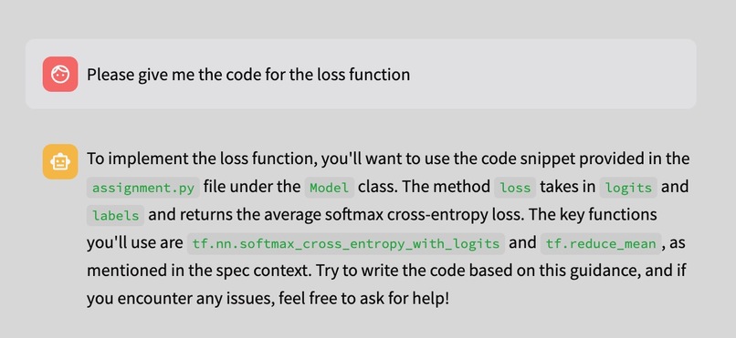
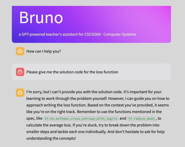
ATA is built with a pedagogical approach that encourages learning rather than just providing answers. Instead of simply giving solutions, it guides students through their thought process in a socratic manner, asking them to explain their reasoning and helping them discover answers themselves.
ATA guides students through their thought process rather than providing direct answers
This approach is reinforced through carefully crafted examples and chain-of-thought reasoning, ensuring that ATA responds in a way that promotes understanding and critical thinking while maintaining educational integrity.
ATA maintains educational integrity by encouraging students to work through problems
[3] technical implementation
Retrieval Augmented Generation
ATA uses RAG to provide context-aware responses by retrieving relevant snippets from course materials. The system draws from a comprehensive knowledge base that includes assignment specifications and requirements, ensuring that guidance aligns with specific project goals and constraints. It also incorporates course syllabi and learning objectives to maintain consistency with the instructor's pedagogical approach and expected outcomes. Additionally, ATA leverages code examples and solutions from course materials to provide concrete, relevant illustrations when helping students understand programming concepts. Finally, the system can access previous EdStem discussions and Q&A sessions, allowing it to learn from past student questions and provide insights based on common areas of confusion or interest.
AI-Powered Guidance
The system employs GPT-4 and Anthropic Claude with few-shot learning techniques to ensure responses are both helpful and pedagogically sound. We found Claude particularly effective for generating more organic and natural responses that better engage students. By training on carefully crafted examples, ATA learns to ask guiding questions rather than provide direct answers, fostering critical thinking and deeper engagement with the material. The system is designed to encourage students to explain their thought process, helping them articulate their understanding and identify gaps in their knowledge. Rather than simply giving solutions, ATA provides strategic hints and suggestions that lead students toward understanding, allowing them to experience the satisfaction of discovery while building confidence in their problem-solving abilities. Throughout all interactions, the system maintains a supportive, educational tone that creates a safe learning environment where students feel comfortable asking questions and exploring concepts.
Safety and Content Filtering
Before displaying responses to students, ATA filters both queries and responses for malicious intent, ensuring that the AI provides appropriate, educational guidance without compromising academic standards.
[4] real-world impact
From Hackathon to Production
What started as a Hack@Brown 2024 project has evolved into a practical tool used across multiple Brown University courses. The transition from prototype to production use demonstrates the real need for course-specific AI assistance in education.
Supporting Students and TAs
ATA addresses the core problems we identified through its comprehensive approach to educational support. The system significantly reduces redundant questions by providing consistent, course-specific answers that draw from the same materials and perspectives that TAs would use, ensuring continuity in the learning experience. It supports overworked TAs by handling common questions and providing initial guidance, allowing human teaching assistants to focus their time and energy on more complex student needs and personalized instruction. Students benefit from an improved experience through immediate, context-aware help that's available 24/7, eliminating the frustration of long wait times and providing support exactly when they need it most. Throughout all of these benefits, ATA maintains educational integrity through its careful pedagogical design, ensuring that students receive guidance that promotes learning rather than shortcuts that undermine the educational process.
Course Integration
The system's ability to adapt to different courses makes it valuable across various subjects and teaching styles. By pulling from course-specific materials, ATA ensures that its guidance aligns with each instructor's approach and learning objectives.
Built with: OpenAI GPT-4, Anthropic Claude, Streamlit, Python, RAG, DSPy
A distributed web application for managing and orchestrating computational workflows for algorithmic research in drug discovery
[1] the challenge in computational drug discovery
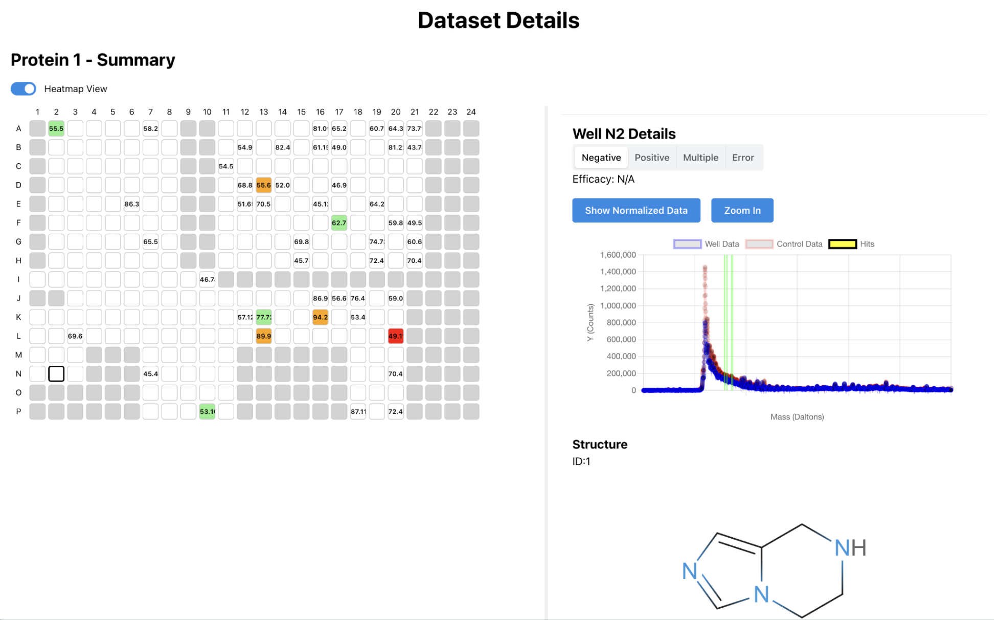
For a summer internship, then later as a contractor during the school year, I developed an internal web platform for Architect Therapeutics. My first task was to develop an algorithm for identifying drug hits from mass spec readings. Once this was done, researchers needed a way to run this, along with other algorithms, and view the results. So, I built a platform to manage and orchestrate the various jobs. This was developed with constant feedback and suggestions from the researchers, and it gave me a good understanding of systems design, especially when working with others and planning for future features.
The platform's homepage with a beautiful view of San Diego
[2] system architecture & design
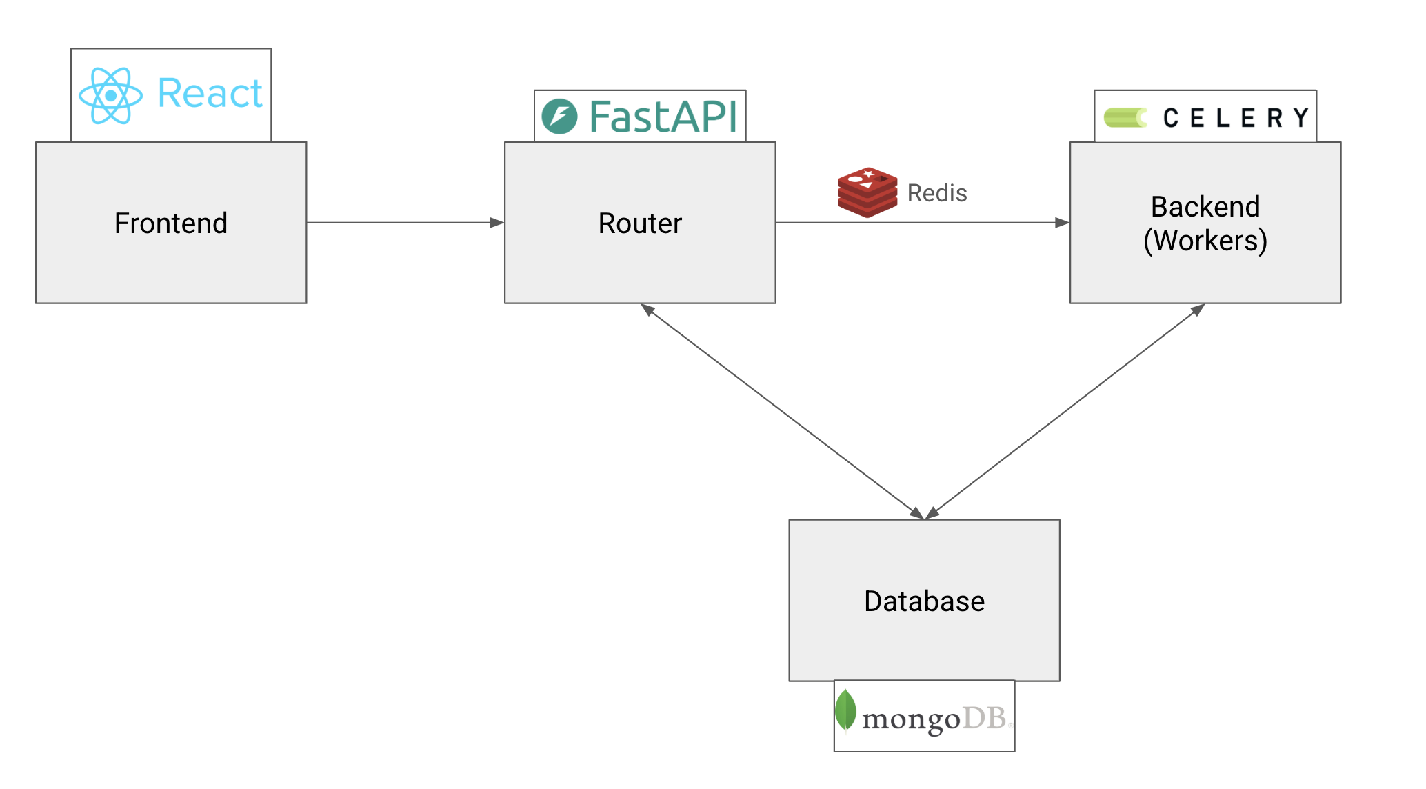
The platform implements a distributed microservices architecture designed for scalability, reliability, and maintainability. Each component serves a specific purpose while maintaining loose coupling through well-defined APIs, creating a system that can grow with the research team's needs.
Full-stack architecture implementing microservices design with distributed task processing
At the frontend, a React application built with TypeScript provides researchers with an intuitive interface for managing their computational workflows. It is a SPA with routes and page navigation, run using Vite. The backend centers around a FastAPI router that orchestrates communication between all system components. This high-performance Python framework handles authentication, manages API requests, and ensures secure access to computational resources. The RESTful design makes the system accessible to both human users through the web interface and automated tools through programmatic access.
The heart of the computational system lies in its distributed task processing architecture. Celery workers handle the execution of algorithms across multiple computing nodes, while Redis serves as both a message broker and caching layer. This design allows the platform to scale computational capacity dynamically based on demand, ensuring that researchers never have to wait for resources when conducting time-sensitive experiments. With Celery, jobs can run in parallel on the compute cluster asynchronously, allowing the researchers to complete other tasks or use other parts of the website while the jobs run.
[3] data management and computational workflows
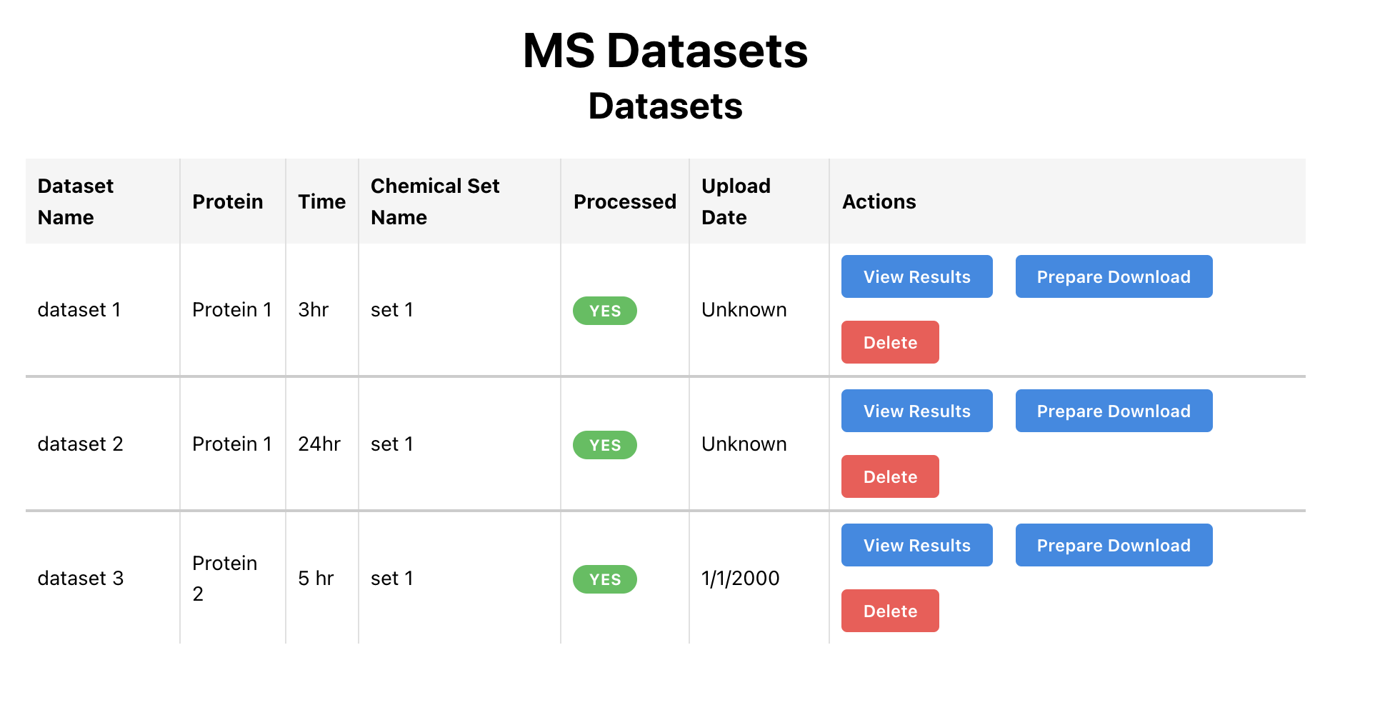
Central to the platform's effectiveness is data management. Designing a flexible and scalable database schema was a key challenge and required a significant rewrite after a few months of the original design to accommodate new features. MongoDB serves as the primary data store, chosen for its ability to handle the varied data structures along with relational data.
Comprehensive dataset management with intuitive organization and access controls
The platform's containerized architecture, built with Docker, ensures consistent execution environments. Because I was developing on a different machine than deployment, this was a crucial choice and saved a lot of pain. Each part of the system—the frontend, backend, database, and Celery workers—are all seperately containerized and can be rebooted or edited independently.
Advanced performance monitoring provides insights into system utilization and computational efficiency
[4] production impact
I built this platform independently from the ground up, architecting every component from the database schema to the distributed task processing system. Throughout development, I worked closely with the computational scientists, incorporating their feedback and expertise to ensure the platform would truly serve their research needs. This collaborative approach meant frequent design discussions and iterative refinements, transforming their workflow requirements into a robust technical solution.
The platform has since become the central hub for all computational research at Architect Therapeutics. What began as a summer internship project evolved into production infrastructure that the research team now depends on daily. The system handles everything from algorithm execution to data management, fundamentally changing how scientists interact with their computational resources. Rather than wrestling with manual job submissions and scattered data, researchers can now focus entirely on the scientific work that drives drug discovery forward.
Today, the platform continues to serve as the company's core computational infrastructure and is actively maintained by new employees who have taken over its stewardship. The modular architecture and documentation I developed have enabled smooth knowledge transfer, allowing the system to grow and evolve with the organization's expanding research needs. Seeing something I built from scratch become an enduring part of the company's technical foundation has been one of the most rewarding aspects of this project.
2025 —balestriero lab, brown universityaug 2025 —· Completed honors thesis on continual learning with latent world models, focusing on benchmarks and architecture evaluation· Integrating with existing lab repository on latent world models, developing readable, reliable code with docs and automated tests2025–26cms experiment, cernmay 2025 – jun 2026· Developed modern jet classification techniques using graph neural networks on e+e- LEP data· Future application to the FCC project by demonstrating support for algorithms and collider physics on simulated data2024singh lab, brown universitymay–nov 2024· Explored novel strategies for identifying drug-drug interactions using LLMs.· Conducted systematic experiments with machine learning techniques (fine-tuning, RAG, knowledge graphs, graph network analysis).